3.2 Estimating clock drift: Permutation
For correcting clock drift, we need to first provide some reasonably good guesses of the true drift values.
permute_clock_drift() can take care of this using a brute-force approach.
For each clock time and receiver pair combination, a series of plausible drift values will be permuted over. For these drift values, an alignment score will be calculated indicating how well the emission and detection events line up between the receivers when this drift has been taken into account. The drift value with the highest alignment score will be returned for that receiver pair and clock time.
There are two available methods for measuring how well the emissions and detections line up and both have their particular use case.
- xcorr: Emission and detection events are represented as Gaussian kernels placed along two time-series (one for each receiver). Cross correlation is applied and the most likely drift value is the one which results in the most overlap between these emission and detection kernels (i.e. the highest cross-correlation score).
- likelihood: Emissions are arranged in a time-series and a mixed detection error distribution is placed over each emission event. Detections are then sampled from this and the joint likelihood that all detection events resulted from any emission event is returned for each drift value. The drift value resulting in the maximum likelihood is chosen.
The above methods can also be used for time-difference-of-arrival detections. That is, sync-tag detections on the receiver pair which are emitted from another receiver in the array.
The xcorr method is preferred if some emission events may be missing from the dataset. However, if there are more reflections than direct detections between the receiver pair, this method risks using the late-arriving reflected sync-tag transmissions to select the drift values.
Conversely, the likelihood method directly accounts for the presence of reflections by treating the detection error as a mixed distribution (see ?ddetect()).
This method assumes that all detection events have a corresponding emission event.
If a few emission events are missing from the dataset, this can cause low likelihood scores.
Both methods are coded by treating the underlying math as convolution operations in the Fourier domain, hence they run extremely fast for the amount of data they process. These work well for getting values on the scale of, say, 0.1 second resolution.
In the following examples, we’ll mostly stick with the default parameters for the xcorr and likelihood methods. These should work fine for most use cases. For more information on how to make use of these optional parameters, see Campbell et al. (in prep) for a detailed description of these methods.
Below, we’ll use the xcorr method.
For each clock_time, we’ll check possible drift values using sync-tag emissions/detections from within a 1 hour-period (the clock_window) centered around each clock_time.
int_drft_xcor <- permute_clock_drift(
  sync_model,
  method = "xcorr",# Evaluate emission/detection alignment with cross-correlation
  clock_resolution = 0.1,# (s) Resolution of the emission/detection time-series
  clock_window = 60*60*1,# (s) Length of window to estimate drift values from
  quiet = T)
print(int_drft_xcor)
## Clock drift permutation values
## Receiver pair: 3 ⟷ 1
## Drift (s) xcorr
## 2021-05-08 18:00:00 0.4 0.95
## 2021-05-08 19:00:00 0.4 0.96
## 2021-05-08 20:00:00 0.4 0.92
## 2021-05-08 21:00:00 0.4 0.94
## 2021-05-08 22:00:00 0.4 0.91
## 2021-05-08 23:00:00 0.4 0.93
## 2021-05-09 00:00:00 0.4 0.93
## 2021-05-09 01:00:00 0.4 0.87
## 2021-05-09 02:00:00 0.5 0.89
## 2021-05-09 03:00:00 0.5 0.88
## 2021-05-09 04:00:00 0.5 0.90
## 2021-05-09 05:00:00 0.5 0.90
## 2021-05-09 06:00:00 0.5 0.91
##
## Receiver pair: 3 ⟷ 2
## Drift (s) xcorr
## 2021-05-08 18:00:00 33.2 0.90
## 2021-05-08 19:00:00 33.3 0.93
## 2021-05-08 20:00:00 33.4 0.85
## 2021-05-08 21:00:00 33.5 0.92
## 2021-05-08 22:00:00 33.5 0.84
## 2021-05-08 23:00:00 33.6 0.88
## 2021-05-09 00:00:00 33.7 0.90
## 2021-05-09 01:00:00 33.8 0.84
## 2021-05-09 02:00:00 33.9 0.83
## 2021-05-09 03:00:00 33.9 0.87
## 2021-05-09 04:00:00 34.0 0.84
## 2021-05-09 05:00:00 34.1 0.83
## 2021-05-09 06:00:00 34.1 0.89
##
## Receiver pair: 3 ⟷ 4
## Drift (s) xcorr
## 2021-05-08 18:00:00 34.6 0.96
## 2021-05-08 19:00:00 34.7 0.96
## 2021-05-08 20:00:00 34.8 0.87
## 2021-05-08 21:00:00 34.8 0.91
## 2021-05-08 22:00:00 34.9 0.91
## 2021-05-08 23:00:00 35.0 0.92
## 2021-05-09 00:00:00 35.1 0.87
## 2021-05-09 01:00:00 35.2 0.86
## 2021-05-09 02:00:00 35.3 0.90
## 2021-05-09 03:00:00 35.3 0.82
## 2021-05-09 04:00:00 35.4 0.80
## 2021-05-09 05:00:00 35.5 0.83
## 2021-05-09 06:00:00 35.6 0.83
##
## Receiver pair: 3 ⟷ 5
## Drift (s) xcorr
## 2021-05-08 18:00:00 30.1 0.94
## 2021-05-08 19:00:00 30.2 0.93
## 2021-05-08 20:00:00 30.3 0.86
## 2021-05-08 21:00:00 30.3 0.92
## 2021-05-08 22:00:00 30.4 0.93
## 2021-05-08 23:00:00 30.5 0.93
## 2021-05-09 00:00:00 30.5 0.90
## 2021-05-09 01:00:00 30.6 0.83
## 2021-05-09 02:00:00 30.7 0.88
## 2021-05-09 03:00:00 30.8 0.82
## 2021-05-09 04:00:00 30.9 0.90
## 2021-05-09 05:00:00 30.9 0.88
## 2021-05-09 06:00:00 31.0 0.89
##
## Receiver pair: 4 ⟷ 6
## Drift (s) xcorr
## 2021-05-08 18:00:00 4.3 0.86
## 2021-05-08 19:00:00 4.3 0.81
## 2021-05-08 20:00:00 4.3 0.75
## 2021-05-08 21:00:00 4.4 0.82
## 2021-05-08 22:00:00 4.3 0.85
## 2021-05-08 23:00:00 4.4 0.78
## 2021-05-09 00:00:00 4.4 0.79
## 2021-05-09 01:00:00 4.4 0.79
## 2021-05-09 02:00:00 4.4 0.78
## 2021-05-09 03:00:00 4.4 0.79
## 2021-05-09 04:00:00 4.4 0.80
## 2021-05-09 05:00:00 4.4 0.78
## 2021-05-09 06:00:00 4.4 0.62Note that larger clock_windows will result in more sync-tag events being used, giving more accurate drift values.
Additionally, lowering the clock_resolution will yield more precise drift values.
The trade-off is that doubling clock_window (or halving clock_resolution) will result in a roughly doubled processing time.
Note that the number of total emissions and detections has no impact on processing times here.
Next we can plot out our estimated drift values.
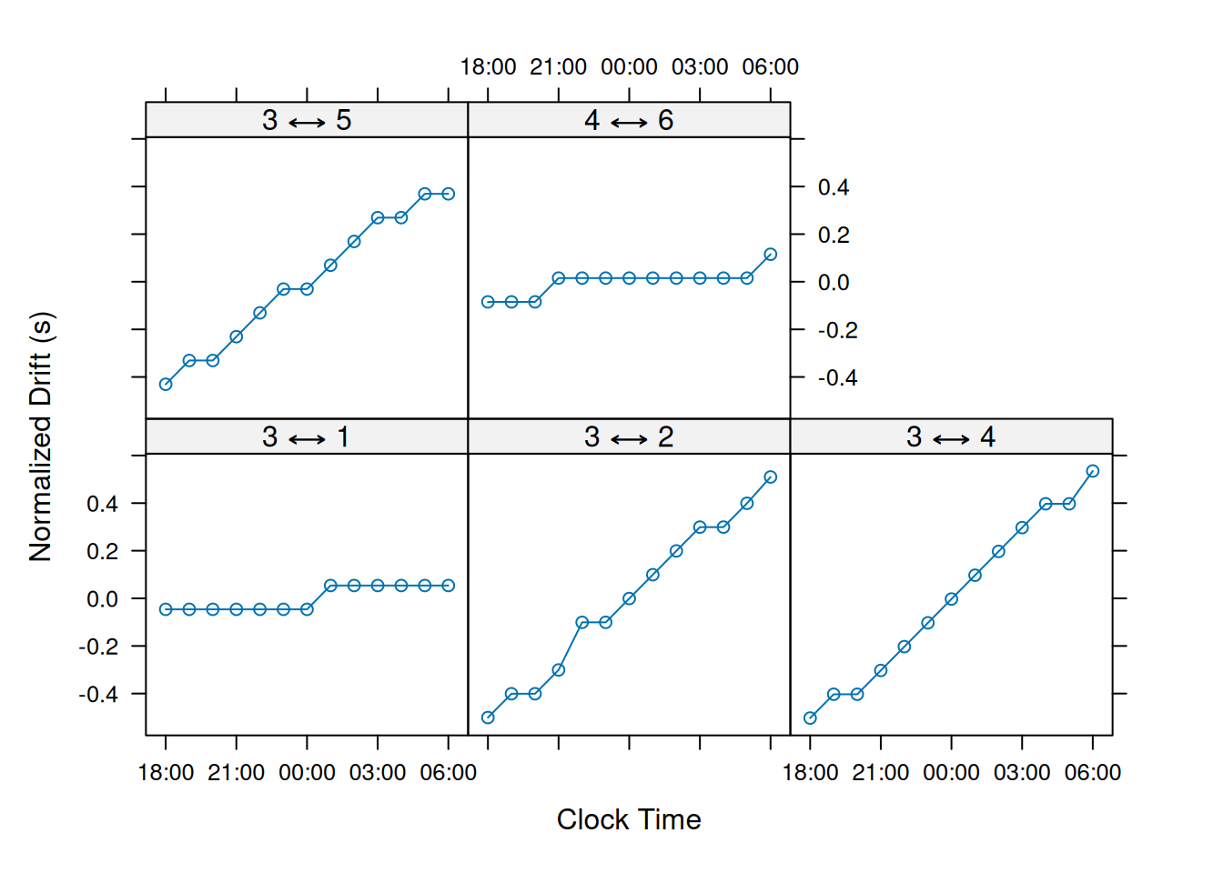
Let’s also do an example of using the likelihood method.
phi is more-less the maximum possible detection error that a late-arriving reflection can result in.
For example, if you expect a tag transmission can travel no father than 1km, then a conservative value for phi can be set with phi = 1000 / 1500.
In other words, we expect reflected transmissions will travel less than one additional kilometer farther than any direct detection.
int_drft_lik <- permute_clock_drift(
  sync_model,
  method = "like",# Evaluate emission/detection alignment with cross-correlation
  clock_resolution = 0.1,# (s) Resolution of the emission/detection time-series
  clock_window = 60*60*1,# (s) Length of window to estimate drift values from
  phi = 1000 / 1500,# (s) Maximum additional latency from reflected detections
  quiet = T)
print(int_drft_lik)
## Clock drift permutation values
## Receiver pair: 3 ⟷ 1
## Drift (s) LogLik.
## 2021-05-08 18:00:00 0.3 0.06
## 2021-05-08 19:00:00 0.3 0.30
## 2021-05-08 20:00:00 0.4 0.20
## 2021-05-08 21:00:00 0.4 0.37
## 2021-05-08 22:00:00 0.4 -0.05
## 2021-05-08 23:00:00 0.4 0.19
## 2021-05-09 00:00:00 0.4 0.26
## 2021-05-09 01:00:00 0.4 0.14
## 2021-05-09 02:00:00 0.4 0.18
## 2021-05-09 03:00:00 0.4 0.08
## 2021-05-09 04:00:00 0.5 0.02
## 2021-05-09 05:00:00 0.5 0.04
## 2021-05-09 06:00:00 0.5 0.20
##
## Receiver pair: 3 ⟷ 2
## Drift (s) LogLik.
## 2021-05-08 18:00:00 33.2 0.15
## 2021-05-08 19:00:00 33.3 0.21
## 2021-05-08 20:00:00 33.3 0.16
## 2021-05-08 21:00:00 33.4 0.32
## 2021-05-08 22:00:00 33.5 0.10
## 2021-05-08 23:00:00 33.6 -0.01
## 2021-05-09 00:00:00 33.7 0.30
## 2021-05-09 01:00:00 33.7 -0.21
## 2021-05-09 02:00:00 33.8 -0.03
## 2021-05-09 03:00:00 33.9 0.04
## 2021-05-09 04:00:00 34.0 -0.45
## 2021-05-09 05:00:00 34.0 -0.45
## 2021-05-09 06:00:00 34.1 0.24
##
## Receiver pair: 3 ⟷ 4
## Drift (s) LogLik.
## 2021-05-08 18:00:00 34.6 0.30
## 2021-05-08 19:00:00 34.6 0.42
## 2021-05-08 20:00:00 34.7 0.27
## 2021-05-08 21:00:00 34.8 0.32
## 2021-05-08 22:00:00 34.9 0.13
## 2021-05-08 23:00:00 35.0 0.19
## 2021-05-09 00:00:00 35.1 0.10
## 2021-05-09 01:00:00 35.1 0.09
## 2021-05-09 02:00:00 35.2 0.25
## 2021-05-09 03:00:00 35.3 0.10
## 2021-05-09 04:00:00 35.4 -0.02
## 2021-05-09 05:00:00 35.5 0.09
## 2021-05-09 06:00:00 35.5 0.34
##
## Receiver pair: 3 ⟷ 5
## Drift (s) LogLik.
## 2021-05-08 18:00:00 30.1 0.30
## 2021-05-08 19:00:00 30.1 0.36
## 2021-05-08 20:00:00 30.2 0.05
## 2021-05-08 21:00:00 30.3 0.49
## 2021-05-08 22:00:00 30.4 0.12
## 2021-05-08 23:00:00 30.5 0.36
## 2021-05-09 00:00:00 30.5 0.34
## 2021-05-09 01:00:00 30.6 0.31
## 2021-05-09 02:00:00 30.7 0.23
## 2021-05-09 03:00:00 30.7 -0.16
## 2021-05-09 04:00:00 30.8 0.28
## 2021-05-09 05:00:00 30.9 0.44
## 2021-05-09 06:00:00 30.9 0.11
##
## Receiver pair: 4 ⟷ 6
## Drift (s) LogLik.
## 2021-05-08 18:00:00 4.3 0.07
## 2021-05-08 19:00:00 4.3 0.34
## 2021-05-08 20:00:00 4.3 -0.20
## 2021-05-08 21:00:00 4.3 0.26
## 2021-05-08 22:00:00 4.3 -0.02
## 2021-05-08 23:00:00 4.3 0.44
## 2021-05-09 00:00:00 4.3 -0.35
## 2021-05-09 01:00:00 4.3 -0.18
## 2021-05-09 02:00:00 4.4 -0.01
## 2021-05-09 03:00:00 4.4 -0.05
## 2021-05-09 04:00:00 4.4 -0.32
## 2021-05-09 05:00:00 4.4 -0.18
## 2021-05-09 06:00:00 4.4 -2.15
Here, the quality of the drift estimates are given by a log likelihood score that is standardized by the number of sync-tag detections. Clock drift values that reduce the detection error will result in relatively higher log likelihood scores which can be compared across receiver pairs.
Now we’ll store our initial drift values in our KaltoaClockSync object.
# Save drift values to KaltoaClockSync model
clock_drift(sync_model) <- int_drft_lik
# Plot sync-tag diagnostics
plot(sync_model, layout = c(4,4))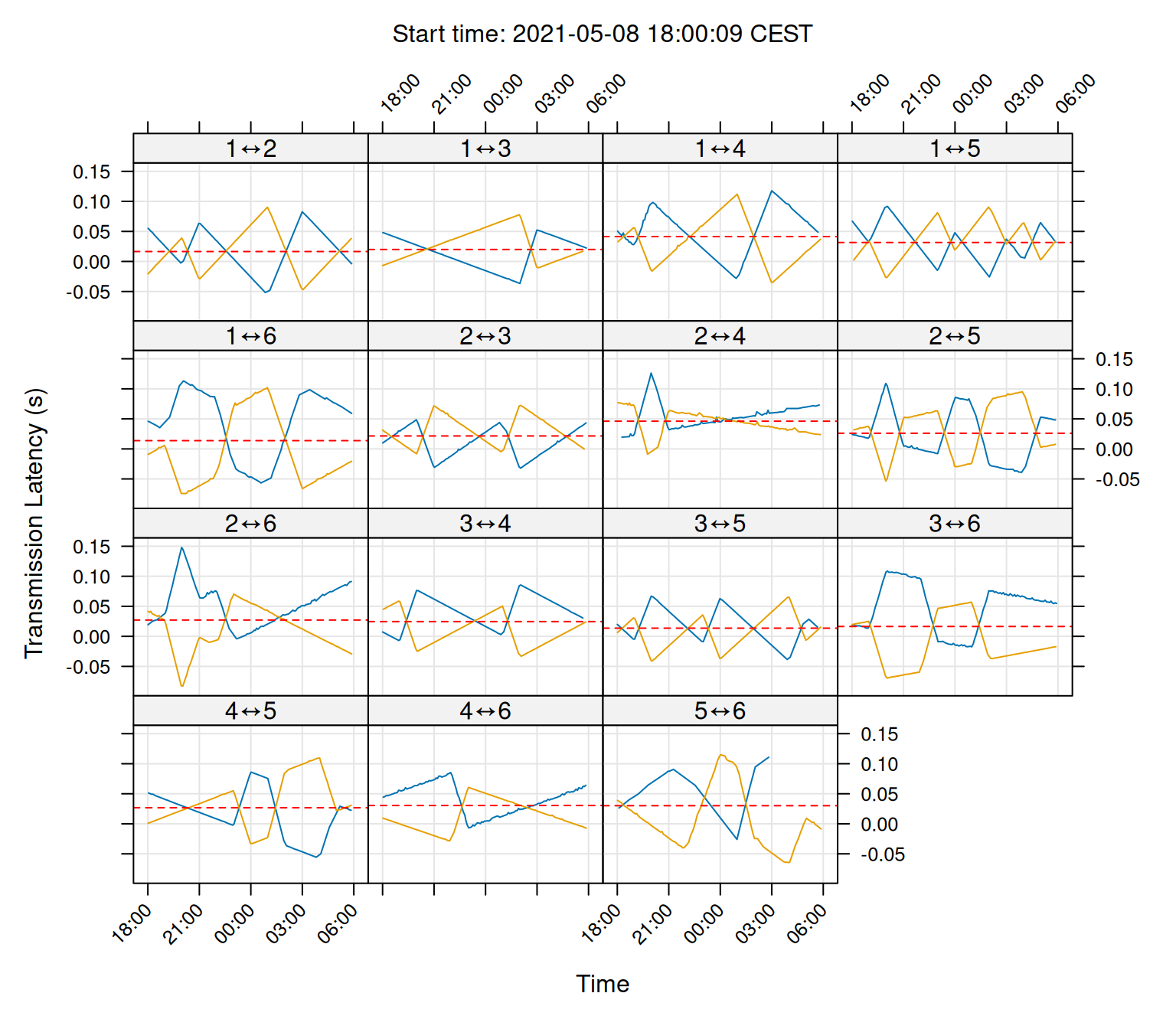
As you can see in the plot, our clocks are roughly corrected within a 0.1 second resolution.
For fine-scale positioning, we’ll need to refine this further using fit_clock_drift.
3.2.1 Cleaning drift estimates
When permute_clock_drift fails to find reasonable drift values, this will result in low xcorr and LogLik. scores.
To solve this, check that (i) clock_window is long enough to capture multiple emission/detection events and (ii) max_drift is set to a high enough value.
For the remaining parameters, the default values should generally be sufficient.
In some cases, the sync-tag data will just be too sparse to estimate a good drift value for a receiver-pair/clock-time. Here, post processing can be done to identify likely incorrect drift estimates and replace them with interpolated values.
First, disable the built-in linear interpolation for missing drift values, permute_clock_drift(..., fit_missing = F).
Missing drift values will now be returned as NaN values.
Next, the code block below gives one example of how the drift values can be cleaned.
# Copy drift values into new object
int_drft_lik_clean <- int_drft_lik
# --- Loop over receiver pairs
for(row in 1:nrow(drift_perm$drift)){
  # --- Remove outliers with robust linear regression
  # Fit model to drift data
  df <- data.frame(
    x = as.integer(clock_times),
    y = int_drft_lik$drift[row,])
  model_linear <- MASS::rlm(y ~ x, data = df)
  # Return fitted drift values
  y_pred <- predict(model_linear, newdata = df)
  # Mark outliers as residuals that exceed 4 standard errors
  idx_rm <- which((abs(y_pred - df$y) /  model_linear$s) > 4)
  # Convert outliers to NA values
  df$y[idx_rm] <- NaN
  # --- Interpolate missing values with GAM
  # Fit a GAM to remaining drift values
  model_interp <- mgcv::gam(y ~ s(x), data = df)
  # Interpolate missing drift values
  idx_na <- which(is.na(df$y))
  df$y[idx_na] <- predict(model_interp, newdata = df[idx_na,])
  # Copy cleaned data back into drift matrix
  int_drft_lik_clean$drift[row,] <- df$y
}
Above, we used a robust linear regression from the MASS package to mark identify and remove likely outliers. Next, we used a generalized additive model from the mgcv package to interpolate the missing data. The best method for outlier detection and drift interpolation will vary per dataset, so kaltoa leaves this up to the user.