3.3 Time-difference-of-arrival (TDOA)

kaltoa uses Smith & Abel’s (1987) spherical interpolation approach for TDOA positioning. This provides a closed form solution to TDOA positioning which is quite fast.

# Apply TDOA positioning
points_tdoa <- TdoaPositioning(
  toa = subset(toa_ppm, detections >= 4 & period < 0.1), 
  remove_outliers = T) 

# Plot results
plot(points_tdoa, sigma_det = sigma_det, main = "TDOA")

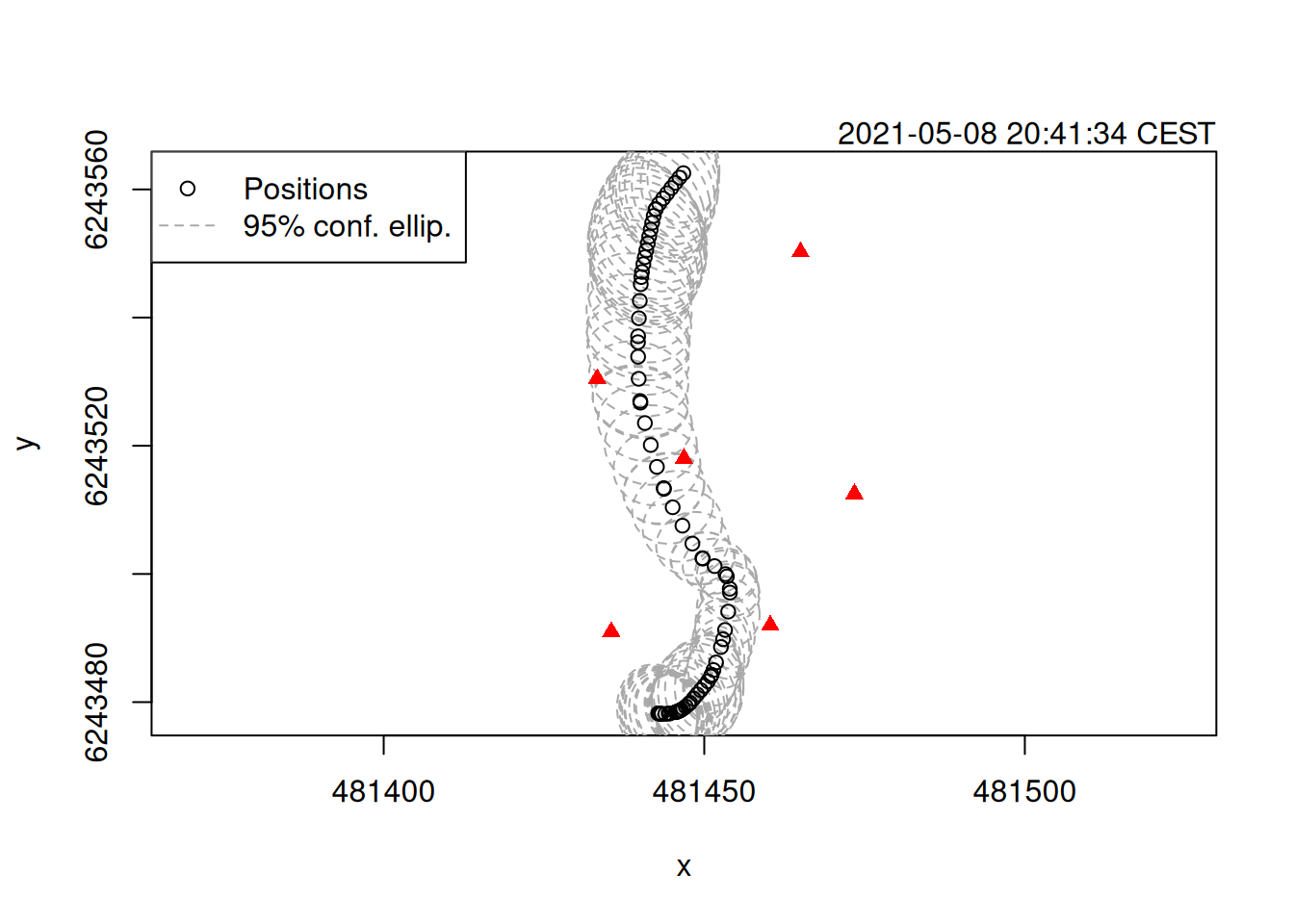
Provided your data has a high volume of detections and your clock data is well calibrated, TDOA positioning can be a very efficient processing option.

When plotting TDOA positions, if the standard deviation of the detection error is supplied a 95% confidence interval will be plotted around each estimate. Note how the positioning uncertainty rises sharply as the tag moves outside of the array. These confidence ellipses are a linear approximation to the true positioning error and can be taken as reasonably accurate if no large outliers are present. Their accuracy has previously been examined in Campbell et al. (2025).

• Campbell, J. A., Shry, S. J., Lundberg, P., Calles, O., Hoelker, F. 2025. A population Monte Carlo model for underwater acoustic telemetry positioning in reflective environments. Methods Ecology and Evolution. 16(4). 775-785.
• Smith, J. and Abel, J. (1987). Closed-form least-squares source location estimation from range-difference measurements. Ieee Transactions Acoust Speech Signal Process 35, 1661–1669.