3.3 Estimating clock drift: Mixed-model
fit_clock_drift will estimate clock drift using a mixed model implemented in TMB.
For each receiver pair, the clock drift is treated a a Gaussian random walk along some linear trend line.
The drift values are fitted as random effects and the detection error is treated as a mixture distribution (see ?ddetect).
For more details on the model, see Campbell et al. (in prep).
This function can provide extremely high resolution drift values.
However, for the model to fit, it requires quite good starting values.
We suggest using permute_clock_drift to get drift values with at least a 0.1 second resolution before applying fit_clock_drift.
fit_drft_1 <- fit_clock_drift(
  sync_model, quiet = T,
  sigma_det = 0.1)# Use clock_resolution as initial detection error value.
print(fit_drft_1)
## --- Kaltoa receiver drift model
## Detection σ (ms) | Drift rate (ms h⁻¹) | Drift σ (ms h⁻¹) | TOA offset (ms) | TDOA offset σ (ms)
## Value, SE | Value, SE | Value, SE | Value, SE | Value, SE
## 3→1 0.096973, 0.0048475 | -6.0588, 10.7521 | 37.246, 7.6027 | -11.1118, 6.4134e-01 | 11.1860, 4.17772
## 3→2 0.323131, 0.0119718 | 5.2923, 12.5535 | 43.487, 8.8768 | -12.9150, 2.7747e+00 | 10.8730, 4.73547
## 3→4 0.242757, 0.0093841 | 9.8687, 12.5215 | 43.376, 8.8541 | 1.3562, 2.4869e-01 | 3.1939, 1.12994
## 3→5 0.269687, 0.0123217 | 7.2397, 13.5902 | 47.078, 9.6100 | -106.2261, 1.1026e+06 | 2.1719, 0.88704
## 4→6 0.876435, 0.0342536 | 1.6109, 7.9652 | 27.592, 5.6333 | -3.1637, 6.0719e-02 | 4.4226, 1.57066
##
## Drift values
## 3→1 3→2 3→4 3→5 4→6
## 2021-05-08 18:00:00 0.38436 33.222 34.583 30.108 4.3173
## 2021-05-08 19:00:00 0.39497 33.303 34.667 30.181 4.3273
## 2021-05-08 20:00:00 0.40566 33.384 34.751 30.255 4.3371
## 2021-05-08 21:00:00 0.41630 33.463 34.836 30.329 4.3468
## 2021-05-08 22:00:00 0.42694 33.544 34.921 30.403 4.3571
## 2021-05-08 23:00:00 0.43751 33.624 35.006 30.477 4.3666
## 2021-05-09 00:00:00 0.44813 33.705 35.091 30.551 4.3771
## 2021-05-09 01:00:00 0.45873 33.785 35.176 30.624 4.3861
## 2021-05-09 02:00:00 0.46934 33.865 35.260 30.699 4.3962
## 2021-05-09 03:00:00 0.47993 33.945 35.345 30.773 4.4059
## 2021-05-09 04:00:00 0.49055 34.026 35.430 30.846 4.4157
## 2021-05-09 05:00:00 0.50106 34.107 35.515 30.920 4.4260
## 2021-05-09 06:00:00 0.51165 34.186 35.601 30.995 4.4367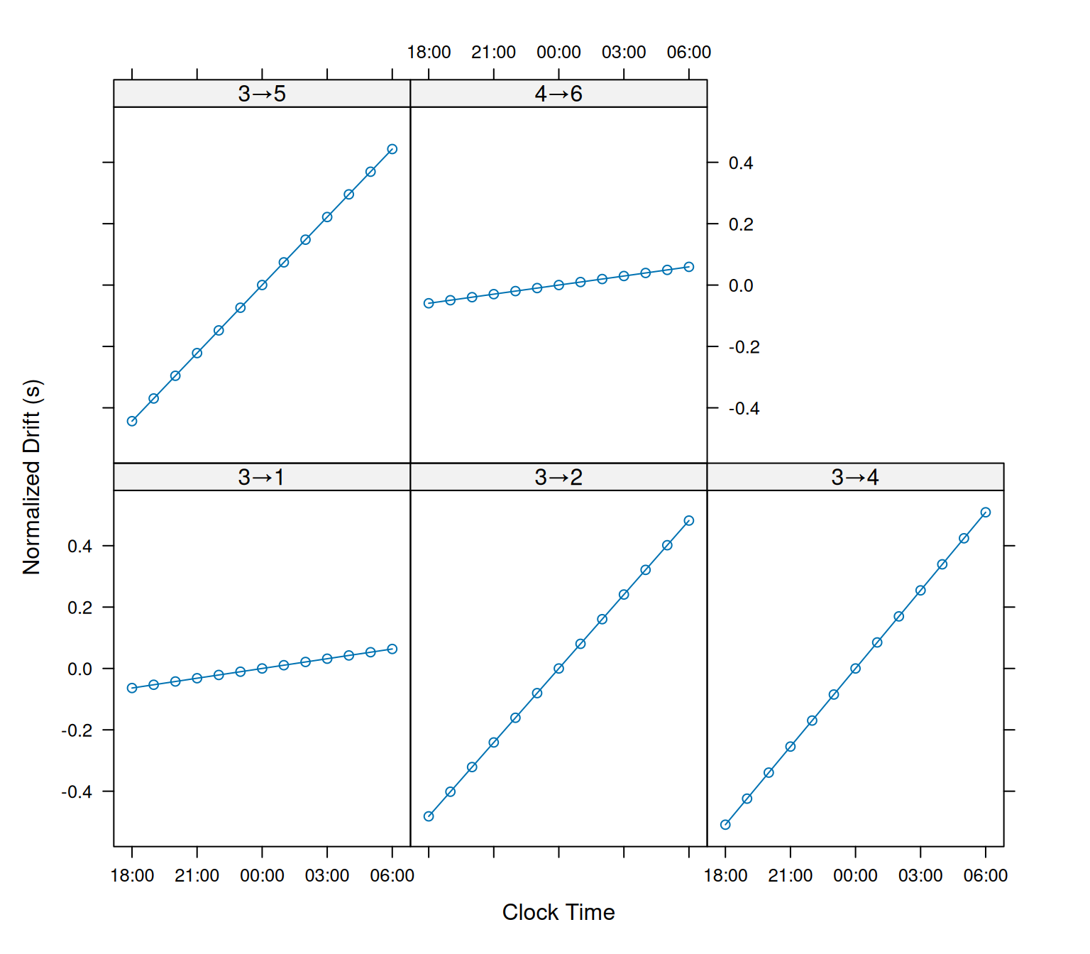
sigma_det is the initial value for the detection error standard deviation (for direct transmissions), in seconds.
It’s recommended to set this to the clock_resolution you used to create the initial drift values.
Setting this too small can cause the model fail.
Fitting these drift values can be a messy process.
There are many parameters being estimated simultaneously by the model, so we often run into problems such as clock drift being mistaken as large detection error values.
To work around this you can opt to fit the model while keeping the inital parameter values fixed.
fix_sigma_det = T tells our model to treat our provided detection error parameter sigma_det = 0.01 as the truth rather than try to estimate it.
Below, we’ll refit the clock drift model a few times using progressively smaller drift error values that are set as fixed values.
sync_model_tmp <- sync_model

fit_drft_tmp <- fit_clock_drift(
  sync_model_tmp, quiet = T,
  sigma_det = 0.1,
  fix_sigma_det = T)# Do not fit the detection error
print(fit_drft_tmp)
## --- Kaltoa receiver drift model
## Detection σ (ms) | Drift rate (ms h⁻¹) | Drift σ (ms h⁻¹) | TOA offset (ms) | TDOA offset σ (ms)
## Value, SE | Value, SE | Value, SE | Value, SE | Value, SE
## 3→1 100, 0 | -6.3424, 10.1967 | 35.539, 11.9931 | -30.154, 4.5947 | 0.0042546, 8.6420
## 3→2 100, 0 | 7.1137, 10.8358 | 37.691, 14.2725 | -33.570, 5.1251 | 0.0045336, 8.7968
## 3→4 100, 0 | 7.4355, 11.5379 | 37.872, 14.9943 | -31.321, 5.5376 | 0.0045014, 8.9664
## 3→5 100, 0 | 4.6309, 10.6210 | 33.256, 22.0223 | -36.604, 7.4902 | 0.0038040, 8.8088
## 4→6 100, 0 | 1.9605, 7.7698 | 27.522, 9.2941 | -33.123, 4.3206 | 0.0049395, 11.9816
##
## Drift values
## 3→1 3→2 3→4 3→5 4→6
## 2021-05-08 18:00:00 0.37687 33.203 34.605 30.132 4.3232
## 2021-05-08 19:00:00 0.36485 33.309 34.649 30.160 4.3289
## 2021-05-08 20:00:00 0.41225 33.352 34.748 30.250 4.3383
## 2021-05-08 21:00:00 0.40617 33.449 34.835 30.328 4.3484
## 2021-05-08 22:00:00 0.41579 33.532 34.921 30.407 4.3580
## 2021-05-08 23:00:00 0.42616 33.613 35.007 30.499 4.3666
## 2021-05-09 00:00:00 0.43691 33.711 35.109 30.529 4.3738
## 2021-05-09 01:00:00 0.44737 33.752 35.157 30.626 4.3659
## 2021-05-09 02:00:00 0.45600 33.853 35.260 30.722 4.4171
## 2021-05-09 03:00:00 0.45007 33.937 35.347 30.751 4.4106
## 2021-05-09 04:00:00 0.49870 34.035 35.434 30.845 4.4177
## 2021-05-09 05:00:00 0.48947 34.076 35.536 30.943 4.4258
## 2021-05-09 06:00:00 0.48837 34.183 35.569 30.962 4.4312# Store fitted drift values
clock_drift(sync_model_tmp) <- fit_drft_tmp
# Refit with a smaller detection error
fit_drft_tmp <- fit_clock_drift(
sync_model_tmp, quiet = T,
sigma_det = 0.01,
fix_sigma_det = T)
print(fit_drft_tmp)## --- Kaltoa receiver drift model
## Detection σ (ms) | Drift rate (ms h⁻¹) | Drift σ (ms h⁻¹) | TOA offset (ms) | TDOA offset σ (ms)
## Value, SE | Value, SE | Value, SE | Value, SE | Value, SE
## 3→1 10, 0 | 1.21669, 5.2695 | 18.195, 3.9915 | 0.33958, 0.67401 | 1.036780, 1.21758
## 3→2 10, 0 | -1.17342, 6.8365 | 23.637, 5.0964 | -1.69391, 0.68364 | 0.000623, 0.87931
## 3→4 10, 0 | 4.23944, 6.5353 | 22.582, 4.9174 | 0.78335, 0.69331 | 2.929212, 1.35373
## 3→5 10, 0 | 4.65450, 8.8010 | 30.449, 6.3877 | -1.31817, 0.69097 | 1.011114, 1.21305
## 4→6 10, 0 | 0.84771, 3.5893 | 12.339, 2.9487 | -3.72734, 0.65634 | 2.884898, 1.99369
##
## Drift values
## 3→1 3→2 3→4 3→5 4→6
## 2021-05-08 18:00:00 0.37362 33.210 34.583 30.108 4.3181
## 2021-05-08 19:00:00 0.38218 33.292 34.666 30.181 4.3274
## 2021-05-08 20:00:00 0.39515 33.371 34.752 30.255 4.3375
## 2021-05-08 21:00:00 0.40417 33.452 34.836 30.329 4.3474
## 2021-05-08 22:00:00 0.41534 33.532 34.921 30.403 4.3577
## 2021-05-08 23:00:00 0.42586 33.612 35.005 30.478 4.3669
## 2021-05-09 00:00:00 0.43652 33.694 35.092 30.551 4.3785
## 2021-05-09 01:00:00 0.44693 33.773 35.175 30.624 4.3838
## 2021-05-09 02:00:00 0.45803 33.854 35.260 30.699 4.3995
## 2021-05-09 03:00:00 0.46724 33.934 35.345 30.772 4.4052
## 2021-05-09 04:00:00 0.48016 34.015 35.429 30.846 4.4160
## 2021-05-09 05:00:00 0.48916 34.094 35.516 30.921 4.4264
## 2021-05-09 06:00:00 0.49973 34.176 35.598 30.993 4.4363# Store fitted drift values
clock_drift(sync_model_tmp) <- fit_drft_tmp
# Refit with a smaller detection error
fit_drft_tmp <- fit_clock_drift(
sync_model_tmp, quiet = T,
sigma_det = 0.001,
fix_sigma_det = T)
print(fit_drft_tmp)## --- Kaltoa receiver drift model
## Detection σ (ms) | Drift rate (ms h⁻¹) | Drift σ (ms h⁻¹) | TOA offset (ms) | TDOA offset σ (ms)
## Value, SE | Value, SE | Value, SE | Value, SE | Value, SE
## 3→1 1, 0 | 0.087824, 0.34710 | 1.19479, 0.29190 | 0.86863, 0.066411 | 1.8789, 0.66880
## 3→2 1, 0 | -0.129854, 0.33156 | 1.14001, 0.29356 | -1.13394, 0.068089 | 1.3301, 0.47816
## 3→4 1, 0 | 0.217449, 0.37508 | 1.28989, 0.32564 | 1.35362, 0.068263 | 3.2206, 1.14124
## 3→5 1, 0 | 0.089719, 0.21491 | 0.73057, 0.22615 | -0.77221, 0.068088 | 1.7872, 0.63602
## 4→6 1, 0 | 0.155110, 0.58428 | 2.01419, 0.46396 | -14.25947, 2.448395 | 7.4147, 3.52989
##
## Drift values
## 3→1 3→2 3→4 3→5 4→6
## 2021-05-08 18:00:00 0.37257 33.211 34.582 30.107 4.3283
## 2021-05-08 19:00:00 0.38281 33.291 34.666 30.181 4.3382
## 2021-05-08 20:00:00 0.39386 33.371 34.752 30.255 4.3481
## 2021-05-08 21:00:00 0.40423 33.452 34.836 30.329 4.3577
## 2021-05-08 22:00:00 0.41502 33.532 34.921 30.403 4.3683
## 2021-05-08 23:00:00 0.42555 33.612 35.006 30.477 4.3777
## 2021-05-09 00:00:00 0.43622 33.693 35.091 30.551 4.3885
## 2021-05-09 01:00:00 0.44671 33.773 35.175 30.625 4.3969
## 2021-05-09 02:00:00 0.45740 33.853 35.260 30.699 4.4077
## 2021-05-09 03:00:00 0.46780 33.934 35.345 30.772 4.4166
## 2021-05-09 04:00:00 0.47871 34.014 35.430 30.846 4.4269
## 2021-05-09 05:00:00 0.48898 34.094 35.515 30.920 4.4372
## 2021-05-09 06:00:00 0.49974 34.175 35.599 30.994 4.4483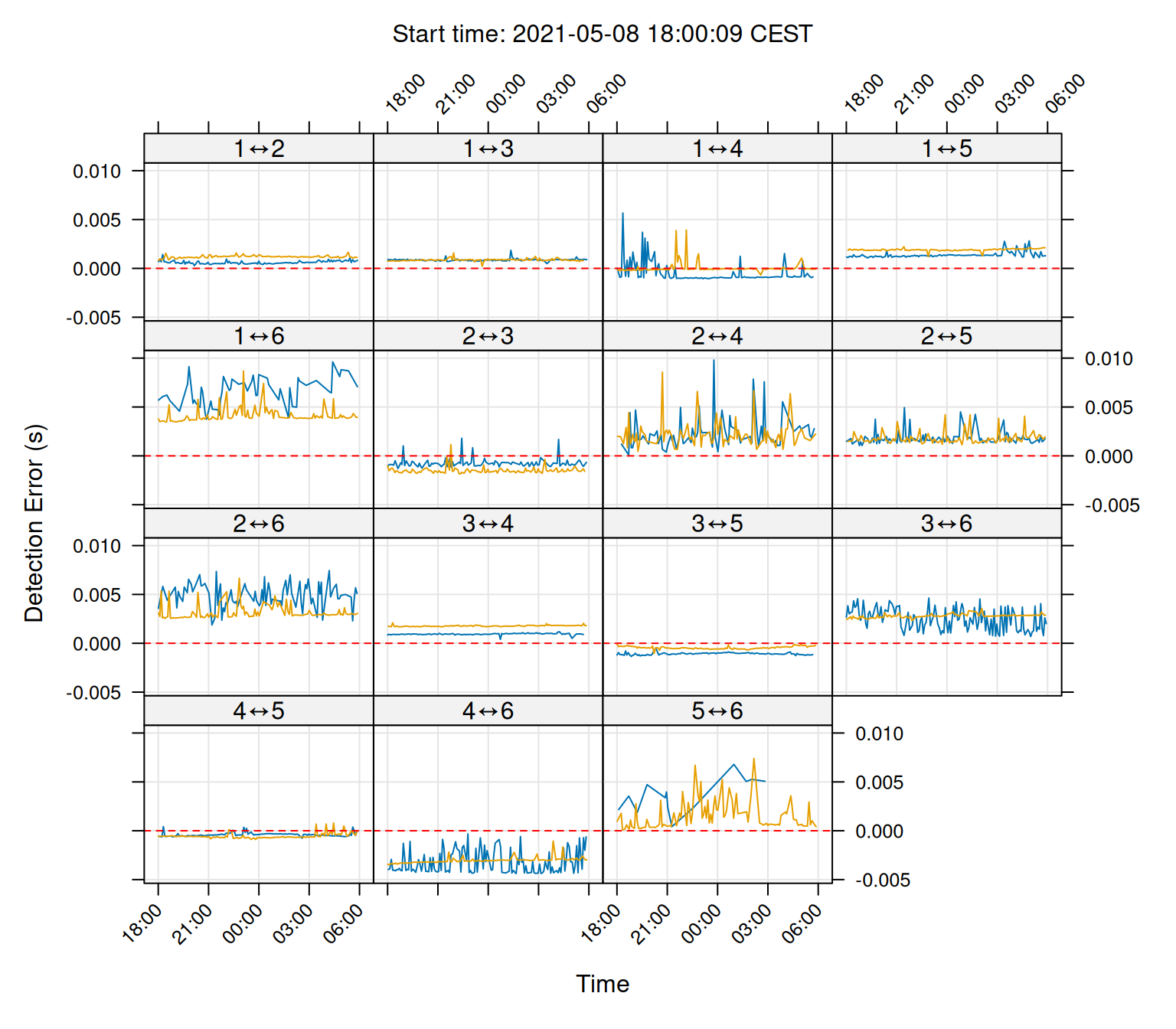
The above method of iteratively fitting smaller fixed values should be seen as a last resort. It’s a messy way to get rough drift values when the model otherwise won’t fit.
Every telemetry array is unique, so some trial and error will have to be used to find which fitting approach works best for the dataset on hand.
Finally, lets store our fitted drift values in our KaltoaClockSync model.
# Save drift values to KaltoaClockSync model
clock_drift(sync_model) <- fit_drft_1
# Plot sync-tag diagnostics
plot(sync_model, type = 'error', layout = c(4,4))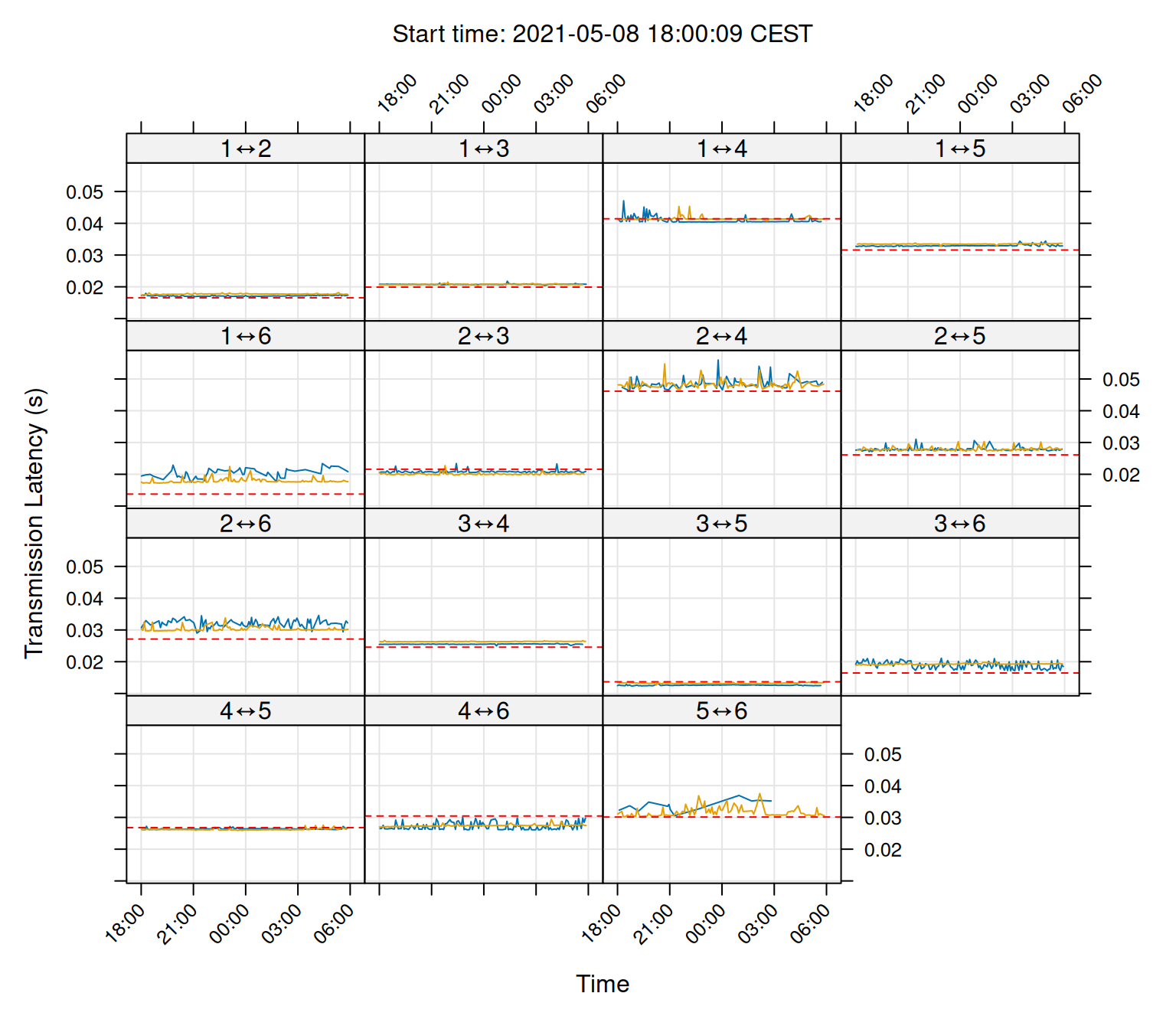

Now the sync-tag diagnostic plots show that the transmission latency is more-less constant over time. Note how some receiver pairs have a bias above or below their expected transmission latencies. These can be corrected for in the next section.
3.3.1 Processing times
Unlike permute_clock_drift, the processing time of fit_clock_drift will be roughly proportional to the number of emissions/detections in the dataset.
For large datasets, we have two suggestions to speed up processing:
- Often, composite tags are used which are a combination of high and low temporal resolution tags—such as 1-2 second interval tag paired with a 1-2 minute interval tag.
Here, we suggest applying
fit_clock_driftto only the low resolution tag. TheDetectionsListin theKaltoaClockSyncmodel can be subset withdetections_list(sync_model) <- detections_list(sync_model) |> subset(type %in% c("PPM", "PPM_SELF")), for example. fit_clock_driftsupports parallel processing. See the sectionMultithreadingin this user guide for mode details.