3.4 Correcting receiver coordinates

The function fit_receiver_positions will try to estimate the true receiver positions. Here, receivers will be moved around until the mean sync-tag transmission latencies for each receiver pair matches well with the expected values. The function simply fits receiver position offset values using R’s optim function.

For this to work, we have to first select at least two receivers as our reference points with ref_receivers. Alternatively, you can specify which receivers you want to estimate offsets for with adj_receivers

# Estimate receiver coordinate offsets
ref_recs = c("2", "5")
pos_offsets <- fit_receiver_positions(sync_model, 
  ref_receivers = ref_recs,
  estimate_transmission_speed = T, 
  estimate_gps_error = F)
# Show results
print(pos_offsets)

## --- Kaltoa receiver position model
## 
## Fitted transmission speed:
## 1397.38 m s⁻¹, SE: 6.65
## 
## Fitted GPS error:
## 0.00 m ⁻¹, SE: 0.00
## 
## Estimated offsets:
##               x offset |   y offset
##             Mean | SE       Mean | SE   
##          1 -0.37   0.19     0.69   0.19 
##          2  0.00   0.00     0.00   0.00 
##          3 -4.59   0.14    -2.37   0.10 
##          4 -2.02   0.22    -3.65   0.21 
##          5  0.00   0.00     0.00   0.00 
##          6  1.73   0.60     6.53   0.65

plot(pos_offsets)

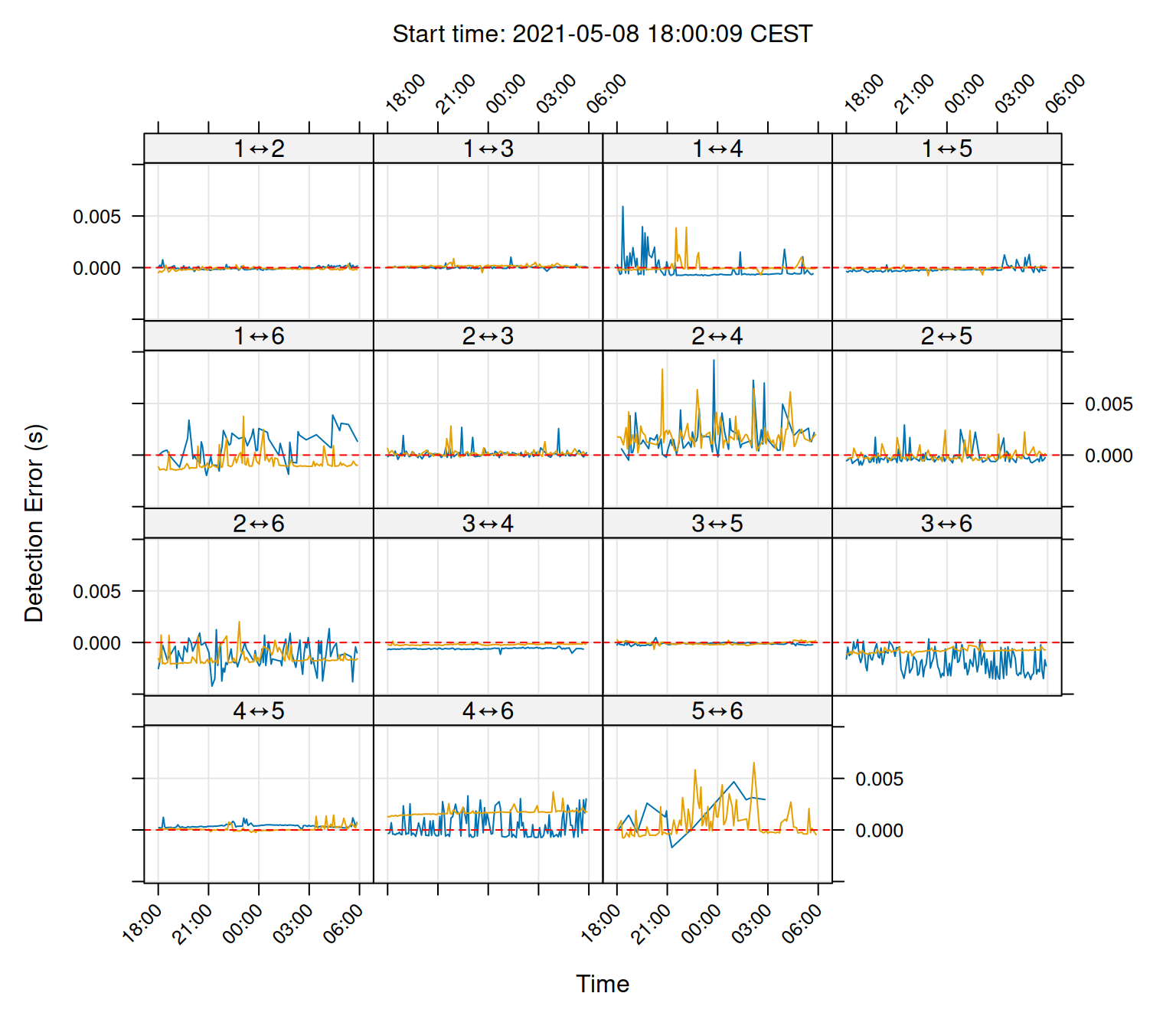
# Save in KaltoaClockSync model
position_offsets(sync_model) <- pos_offsets
# Refit new clock offsets
clock_offsets(sync_model) <- fit_clock_offsets(sync_model, 
  estimate_transmission_speed = F)
# Show newest diagnostic plot
plot(sync_model, type = 'error')

Note how we recalculated our clock_offsets after we applied our new receiver positions. The new distances between receiver pairs will throw off our previous clock_offset estimates.

The final sync-tag latency plot isn’t perfect (and never will be), but it should give us enough precision to apply our positioning models. Generally, you should be pretty happy if you can get your sync-tags corrected to within a 1-2 ms accuracy.