4.5 Kalman Filter: Post-processing

For position estimates returned by TdoaPositioning and KaltoaPMCPositioning, post processing can be applied with a Kalman filter. In this case, KaltoaTrackPositioning will apply a continuous-time correlated random walk (CTCRW; Johnson et al., 2008). This makes use of the positioning error covariances and refines position estimates by making simple assumptions about the animals movement velocity process.

First, you need to set up a KaltoaProcessModel which holds the parameters of the movement model.

# --- Create process model
# Time until velocity correlation falls below 0.05
t_05 = 15# (s)
# Stationary velocity SD
sigma_vel = 0.2# (m/s)
# Setup KaltoaProcessModel object
beta = -log(0.05) / t_05
alpha = sigma_vel * sqrt( 2 * beta )
proc_ctcrw <- KaltoaProcess(type = "ctcrw", alpha = alpha, beta = beta)
plot(proc_ctcrw)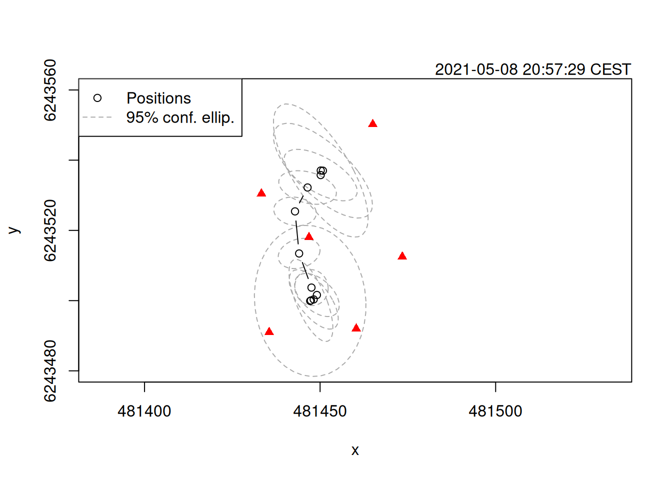

Here, the velocity in each spatial dimension (x or y) is treated as a Ornstein-Uhlenbeck (OU) process. An OU process is more-less a correlated random walk in continuous time. To parameterize this, we’ve specified that we want the velocity correlation (along a given dimension) to fall below 0.05 after 15 seconds. Furthermore, if we were to randomly sample any point along our animal’s track, we’d expect the magnitude of the velocity in the horizontal plane (the length of the summed x and y velocities) to fall along a Rayleigh distribution with a mode of 0.2 meters per second.

Using these parameters, we can place some common-sense restrictions on our animals movement process which will help reign in any poorly-estimated positions.

Now we can apply this movement model to our PMC-TOA results via a Kalman filter.

track_pmc <- KaltoaTrackPositioning(
  x = points_pmc, process_model = proc_ctcrw) |> smooth()
plot(track_pmc)
points(positions(toa_ppm), pch = 17, col = 'red')

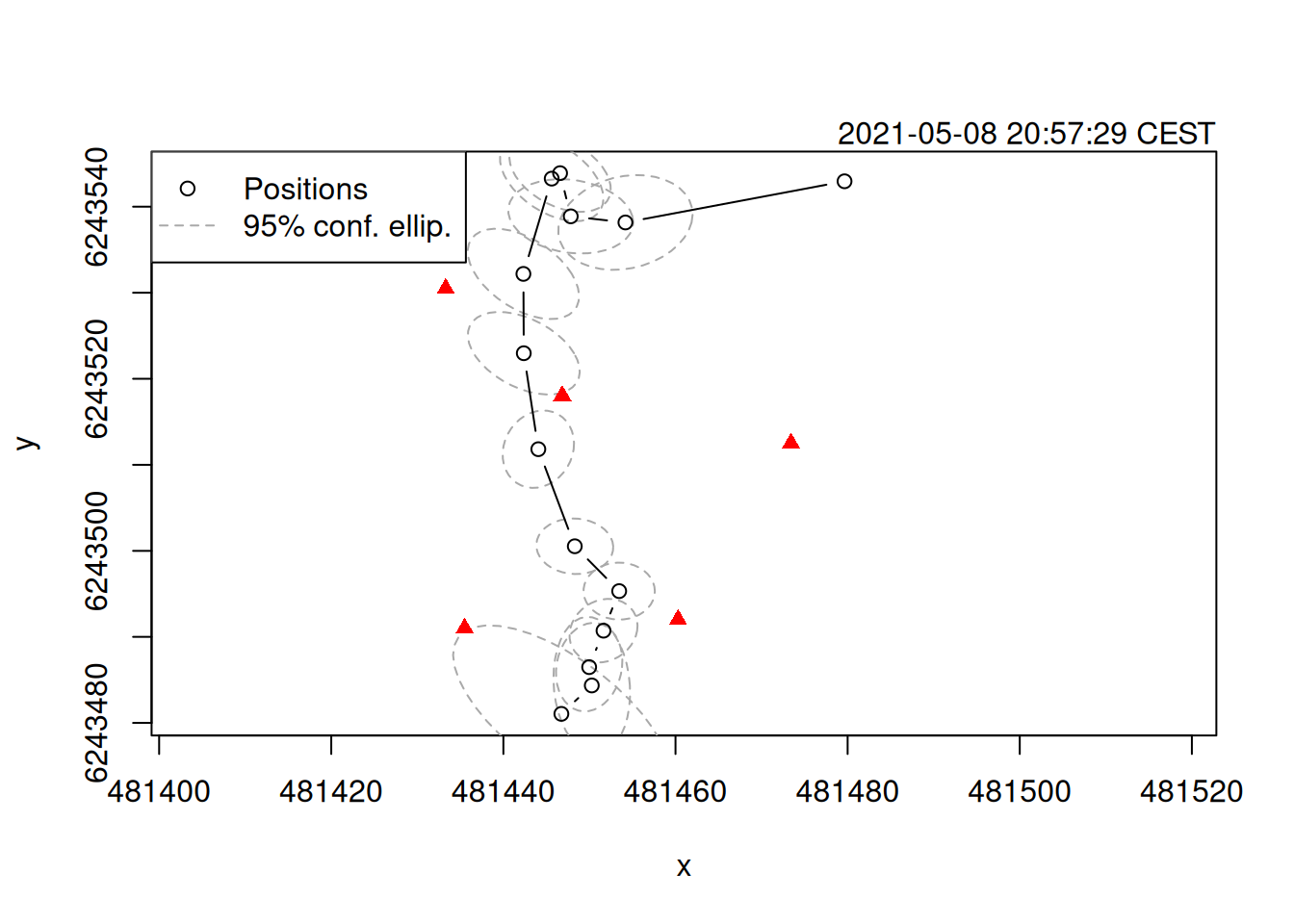
The smooth function applies a Rauch–Tung–Striebel smoother the the estimates. Filtering utilizes previous measures to update current position estimates, while smoothing uses future measures to refine those filtered estimates ever further.

For the sake of completeness, below is the Kalman filtered and smoothed results from our earlier TDOA positioning model.

track_tdoa <- KaltoaTrackPositioning(
  x = as.KaltoaPointPositions(points_tdoa, sigma_det = 0.002), 
  process_model = proc_ctcrw) |> smooth()
plot(track_tdoa, xlim = c(481420, 481500), ylim = c(6243480, 6243560))
points(positions(toa_ppm), pch = 17, col = 'red')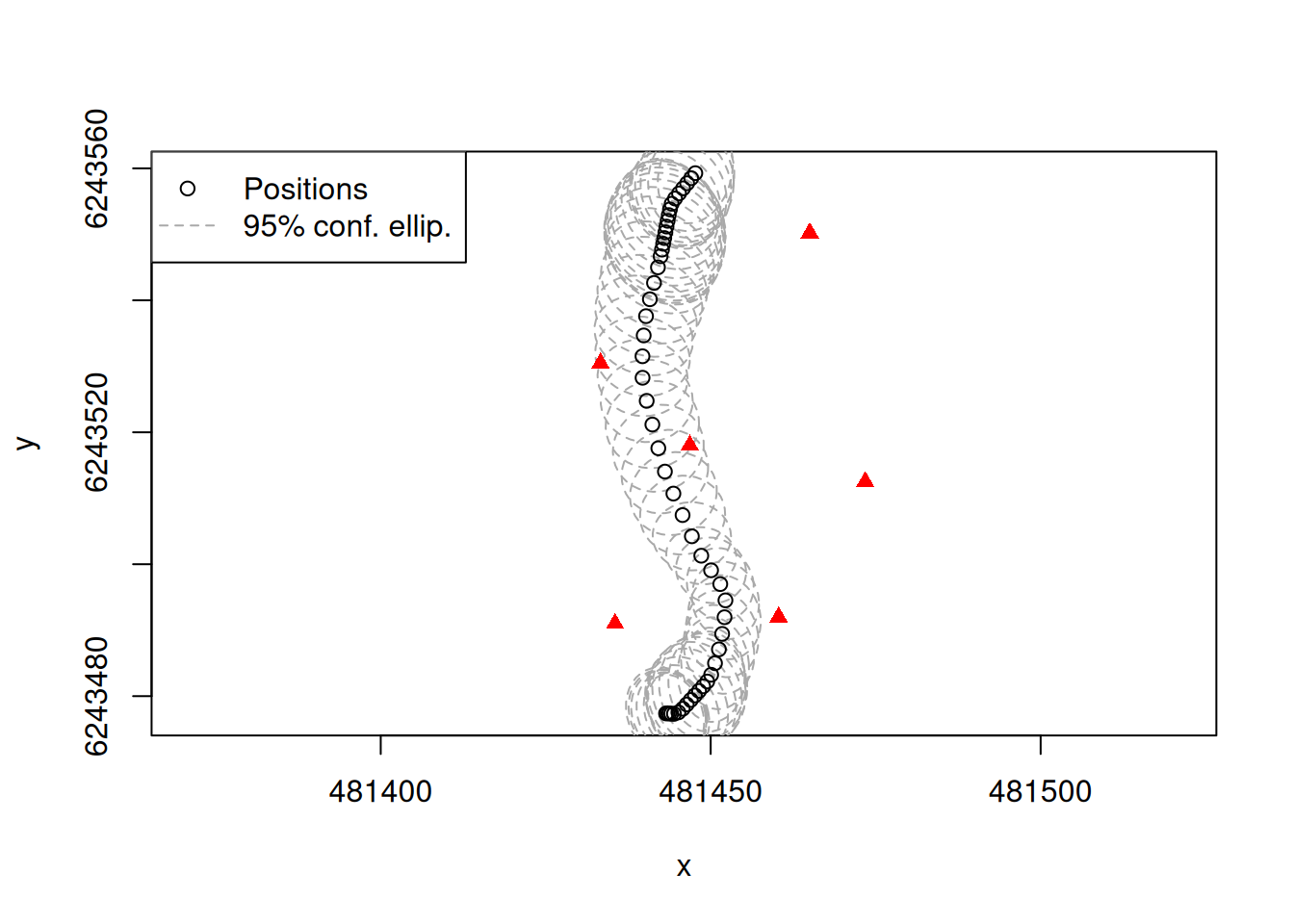

Considering we’re concerned about the presence of reflected detections — which TDOA positioning can’t take into account — we don’t place much trust in these filtered & smoothed estimates. For Kalman filter post processing, it’s crucial that you have a reasonable degree of trust in the error measures (i.e. covariance matrices) attached to your position estimates.

• Johnson, D. S., London, J. M., Lea, M.-A., Durban, J. W. 2008. Continuous-Time Correlated Random Walk Model for Animal Telemetry Data. Ecology, 89(5), 1208–1215.