3.1 KaltoaClockSync
KaltoaClockSync objects hold correction values that can be used to synchronize receiver clocks within an array.
Additionally, it can also hold receiver position corrections.
Below is a plot of our receiver array.
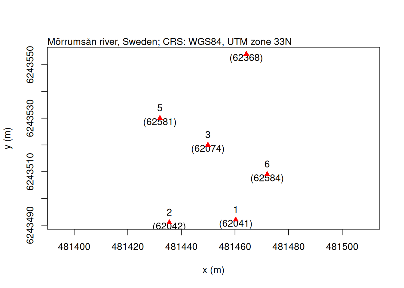
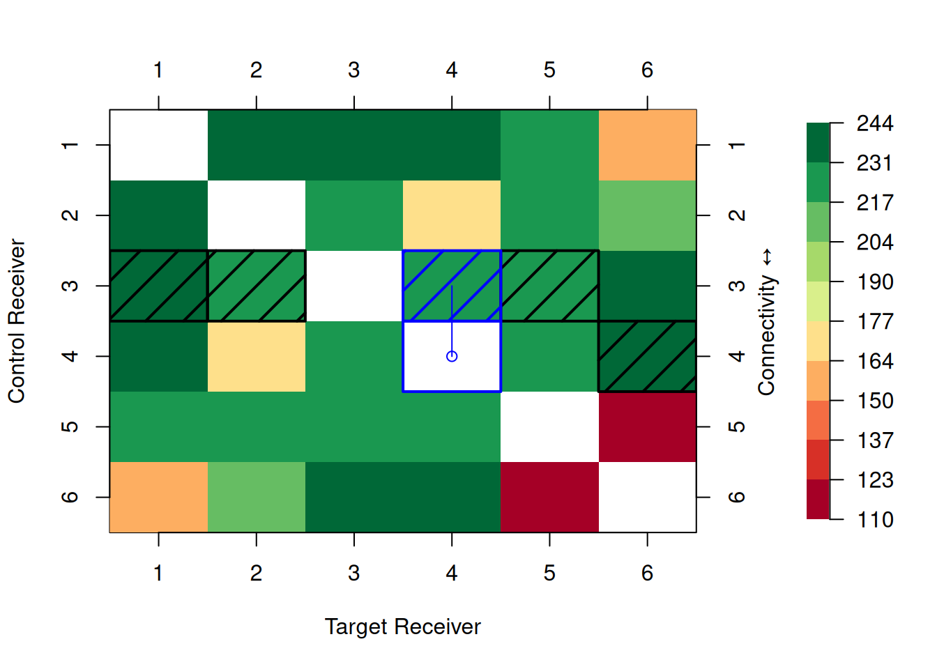
We can use the function SyncTagConnectivity to tally the number of sync-tag detections between receiver pairs.
# Show connectivity
# (number of detections between receiver pairs)
sync_conn <- SyncTagConnectivity(exdata_clocksync)
sync_conn
## $connectivity_matrix
## detect
## emit 1 2 3 4 5 6
## 1 NaN 118 117 117 112 110
## 2 123 NaN 118 95 114 119
## 3 114 107 NaN 110 111 111
## 4 114 78 110 NaN 113 113
## 5 111 106 109 111 NaN 95
## 6 52 89 133 131 15 NaN
##
## $array_attributes
## name emit_id x y depth depth.1
## 1 1 62041 481460.3 6243492 NA NA
## 2 2 62042 481435.5 6243491 NA NA
## 3 3 62074 481449.9 6243520 NA NA
## 4 4 62368 481464.2 6243554 NA NA
## 5 5 62581 481432.0 6243530 NA NA
## 6 6 62584 481472.0 6243509 NA NA
##
## attr(,"class")
## [1] "SyncTagConnectivityMatrix" "list"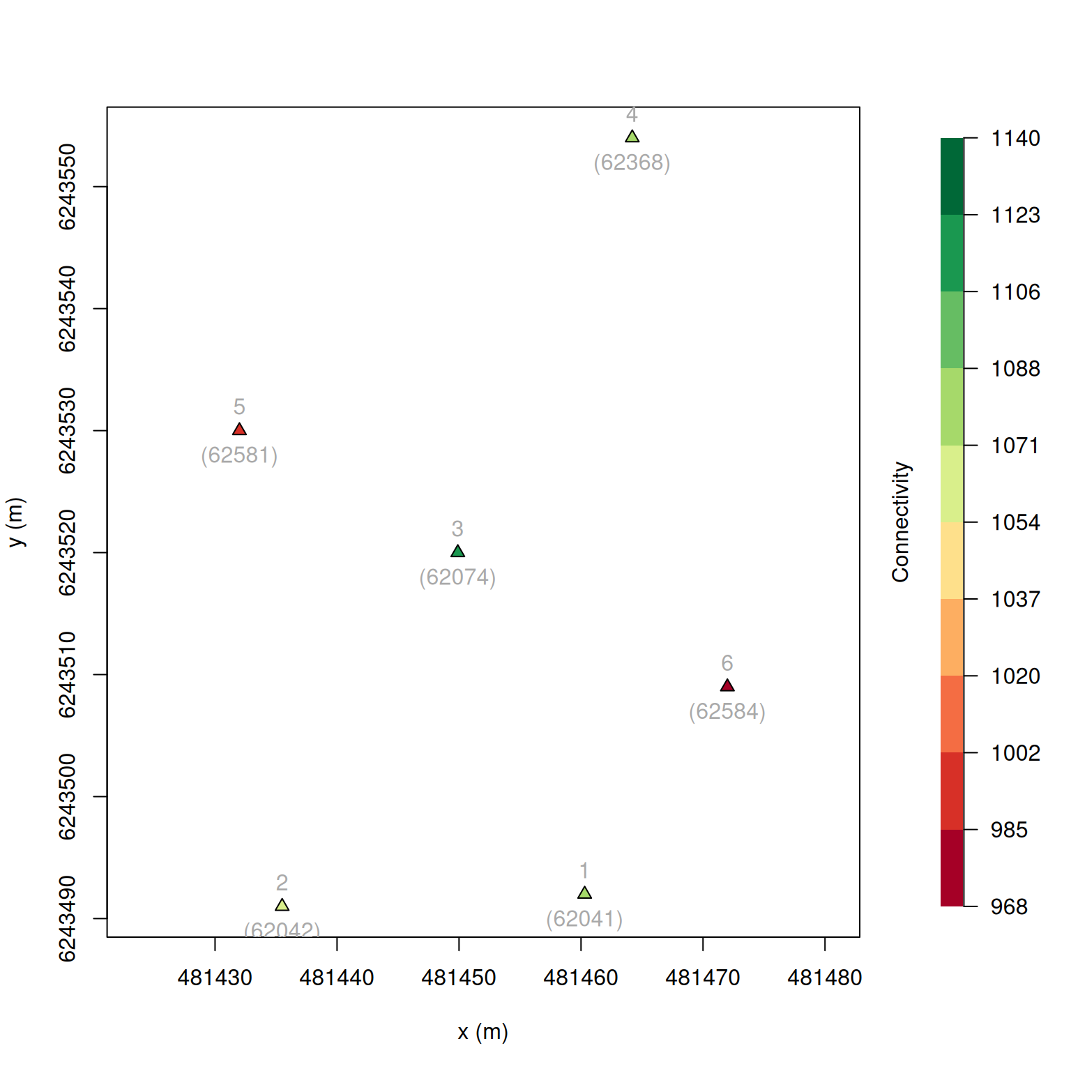
The "map" plot is useful for deciding on your best controller receiver.
That is, the receiver which shares the most sync-tag emissions/detections with all other receivers.
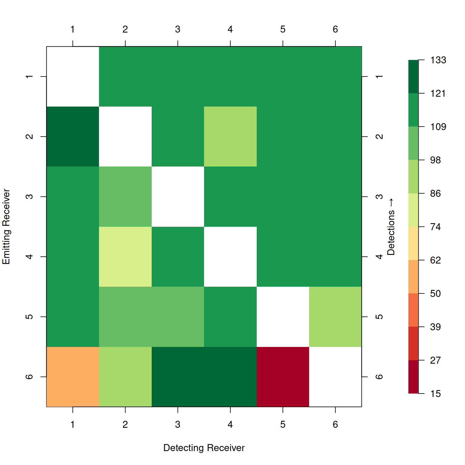
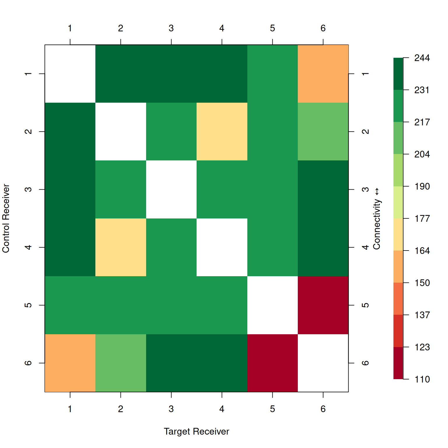
The "matrix" plot is great for identifying weak links in your sync_order.
If one receiver has poor connectivity with your controller, it might be a good idea to add a second controller that has better connectivity to that receiver.
Next, we’ll need to specify a data.frame providing the order for the pairwise clock drift corrections, sync_order.
You can string together calls of the sync_pair function to create a correctly formatted sync_order object.
# Create a data.frame holding the order of paired clock synchronizations
sync_order <-
  sync_pair(
    controller = "3",
    target = c("1", "2", "4", "5")) +
  sync_pair(
    controller = "4", target = "6")
sync_order
## controller target toa_ct toa_tc tdoa_ct
## 1 3 1 TRUE TRUE TRUE
## 2 3 2 TRUE TRUE TRUE
## 3 3 4 TRUE TRUE TRUE
## 4 3 5 TRUE TRUE TRUE
## 5 4 6 TRUE TRUE TRUEHere, receiver 3 will synchronize the rest of the array except for receiver 6.
Next, receiver 4 will be used as a controller to synchronize the remaining receiver 6.
The last three columns indicate which sync-tag detections to include in the synchronization.
toa_ct and toa_tc refer to sync-tag transmissions travelling from the controller to target receiver and vice versa, respectively.
toa_ct can be read as time-of-arrival from controller to target.
tdoa_ct refers to sync tags detected on the receiver pair that are emitted from other receivers in the array.
This can be read as time-difference-of-arrival from controller to target.
For tdoa_ct detections, the emission time is not required.
As a result, sentinel tags placed across the array with known positions can be used here.
Do do this, you can simply make a Detections object for the sentinel tag to treat it as a receiver with no detections.
For larger arrays, you can make use of the fill_sync_order function.
Here, you simply specify a sync_order that only contains potential controller receivers.
fill_sync_order will then attach the remaining receivers to the best connected controller from your sync _order.
# An (convoluted) example of how to specify many controllers
sync_order_alt <-
  sync_pair(controller = "1", target = "3") +
  sync_pair(controller = "3", target = "6") |>
  fill_sync_order(detlst = exdata_clocksync)
sync_order_alt
## controller target toa_ct toa_tc tdoa_ct
## 1 1 3 TRUE TRUE TRUE
## 2 3 6 TRUE TRUE TRUE
## 3 3 1 TRUE TRUE TRUE
## 4 3 2 TRUE TRUE TRUE
## 5 3 5 TRUE TRUE TRUE
## 6 6 4 TRUE TRUE TRUETake your time on setting up the sync_order table and make use of plot(sync_conn, type = "matrix") to verify your choices.
Receivers pairs with poor sync-tag connectivity will result in bad drift corrections.
If possible, it is best to have 1 single well connected receiver acting as a controller for the entire array.
We’ve added a second controller above just for the sake of an example.
We’ll calculate drift corrections on an hourly basis by setting appropriate clock times.
# Make a vector of times to calculate clock drift corrections for.
clock_times <- seq(
  as.POSIXct("2021-05-08 18:00:00", tz = "CET"),
  as.POSIXct("2021-05-09 06:00:00", tz = "CET"), by = 3600)
clock_times
## [1] "2021-05-08 18:00:00 CEST" "2021-05-08 19:00:00 CEST"
## [3] "2021-05-08 20:00:00 CEST" "2021-05-08 21:00:00 CEST"
## [5] "2021-05-08 22:00:00 CEST" "2021-05-08 23:00:00 CEST"
## [7] "2021-05-09 00:00:00 CEST" "2021-05-09 01:00:00 CEST"
## [9] "2021-05-09 02:00:00 CEST" "2021-05-09 03:00:00 CEST"
## [11] "2021-05-09 04:00:00 CEST" "2021-05-09 05:00:00 CEST"
## [13] "2021-05-09 06:00:00 CEST"Next, we’ll create the KaltoaClockSync model.
This holds our parameters for clock synchronization.
To handle reflected transmissions we can use the parameter phi.
A value of phi = 0.33 means that we’re expecting reflected transmissions may be detected up to 0.33 seconds later than their direct-transmission counterparts.
This tells our clock-synchronization models to not be surprised if large positive outliers appear in the data set.
# Transmission are assumed to travel no farther than 500 meters.
# We can use this to set phi (maximum added latency from a reflected
# transmission)
phi <- 500 / 1500

# Initialize model
sync_model <- KaltoaClockSync(
  sync_order = sync_order,
  phi = phi,
  clock_times = clock_times,
  detlst = exdata_clocksync,
  max_drift = 120)
print(sync_model)
## KaltoaClockSync Object
##
## --- Parameters
## Detection error phi: 0.3 s
## Detection error beta: 32.0
## Detection-emission grouping threshold: 0.5 s
## Transmission speed: 1500.0 m s⁻¹
## Max drift: 120.0 s
##
## 13 clock times ranging: 2021-05-08 18:00:00 -- 2021-05-09 06:00:00 (CET)
##
## --- Clock drift ranges
## 3 ⟷ 1: 0.0000 s -- 0.0000 s
## 3 ⟷ 2: 0.0000 s -- 0.0000 s
## 3 ⟷ 4: 0.0000 s -- 0.0000 s
## 3 ⟷ 5: 0.0000 s -- 0.0000 s
## 4 ⟷ 6: 0.0000 s -- 0.0000 s
##
## --- Clock offsets
## 1: 0.0000 s
## 2: 0.0000 s
## 3: 0.0000 s
## 4: 0.0000 s
## 5: 0.0000 s
## 6: 0.0000 s
##
## --- Position offsets
## 1: 0.0 m, 0.0 m
## 2: 0.0 m, 0.0 m
## 3: 0.0 m, 0.0 m
## 4: 0.0 m, 0.0 m
## 5: 0.0 m, 0.0 m
## 6: 0.0 m, 0.0 mThe next sections will deal with using our sync-tag data to estimate the appropriate drift and offset values for this object.