4.1 TOAMatrix
DetectionsList objects can be easily converted into TOAMatrix objects with get_toa.
Detections which match a given tag_id and occur within group_thresh seconds of each other are grouped into emission events for that tag.
The transmission_speed parameter will be later used by the positioning models we’ll apply to this.
toa_hr <- get_toa(exdata_positioning, tag_id = "HR-53883",
  group_thresh = 0.5, transmission_speed = 1420)
summary(toa_hr)
head(toa_hr, 10)
## TOAMatrix
## Tag ID: HR-53883
## Transmission speed: 1420.00 m s⁻¹
## Time zone: CET
## ------ Detections
## First Detection: 2021-05-08 20:41:34
## Last Detection: 2021-05-08 21:29:30
## Reference time: 2021-05-08 20:41:34
## Detection Period: 0.8 hours
## ------ Emissions
## Emissions: 419
## Detections per emission (proportional)
## 1 2 3 4
## 0.48 0.37 0.11 0.03
## ------ Receiver Positions
## x y depth
## 1 481460.3 6243492 NA
## 2 481435.5 6243491 NA
## 3 481446.8 6243518 NA
## 4 481465.0 6243550 NA
## 5 481433.3 6243530 NA
## 6 481473.4 6243513 NA
## 1 2 3 4 5 6 time
## 1 0.5225566 NaN NaN NaN NaN NaN 2021-05-08 20:41:34
## 2 96.7468368 NaN 96.72943 NaN NaN NaN 2021-05-08 20:43:10
## 3 NaN NaN NaN 106.8677 NaN NaN 2021-05-08 20:43:20
## 4 NaN NaN 113.54463 NaN NaN NaN 2021-05-08 20:43:27
## 5 NaN NaN NaN NaN 160.4745 NaN 2021-05-08 20:44:14
## 6 NaN NaN 165.53259 NaN NaN NaN 2021-05-08 20:44:19
## 7 NaN NaN 175.42440 NaN 175.4183 NaN 2021-05-08 20:44:29
## 8 NaN NaN 208.82124 NaN NaN NaN 2021-05-08 20:45:02
## 9 231.3057200 NaN NaN NaN NaN NaN 2021-05-08 20:45:25
## 10 NaN NaN 310.46417 NaN NaN NaN 2021-05-08 20:46:44TOAMatrix objects show relative detection times to make the underlying data more readable.
The reference time stamp (0 seconds) is stored as the attribute "start_time".
In the case of composite tags composed of two tags operating at different frequencies, we can combine these detections into a single TOA matrix.
toa_ppm <- get_toa(exdata_positioning, tag_id = "PPM-53883",
  group_thresh = 0.5, transmission_speed = 1420)
toa_comp <- c(toa_hr, toa_ppm)
summary(toa_comp)
## TOAMatrix
## Tag ID: Multiple tags
## Transmission speed: 1420.00 m s⁻¹
## Time zone: CET
## ------ Detections
## First Detection: 2021-05-08 20:41:34
## Last Detection: 2021-05-08 21:29:30
## Reference time: 2021-05-08 20:41:34
## Detection Period: 0.8 hours
## ------ Emissions
## Emissions: 448
## Detections per emission (proportional)
## 1 2 3 4 5
## 0.48 0.35 0.11 0.04 0.01
## ------ Receiver Positions
## x y depth
## 1 481460.3 6243492 NA
## 2 481435.5 6243491 NA
## 3 481446.8 6243518 NA
## 4 481465.0 6243550 NA
## 5 481433.3 6243530 NA
## 6 481473.4 6243513 NAWhen using c() to combine tags into composite TOA matrices, the results will automatically be time ordered for you.
If the TOAMatrix objects have conflicting metadata, warnings will be shown.
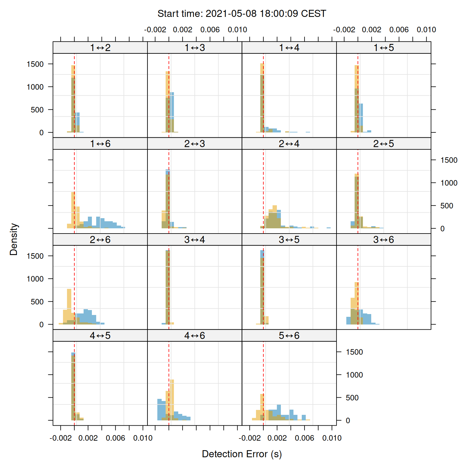
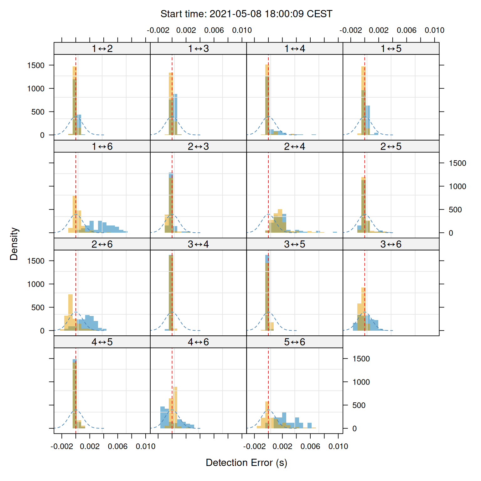
We can use the plot function to get a good overview of what our data set looks like.
Next, we can filter our TOA data using diagnostic measures. The detection period — difference between the first and last detection — can be used to filter out emissions that likely have large detection outliers resulting from multi-path reflections. We can also filter based on the number of detections per emission.
# Filter TOA using diagnostics
toa_filt <- subset(toa_comp, period < 0.1 & detections >= 3)
# Show diagnostics for filtered TOA data
plot(toa_filt, type = "diag")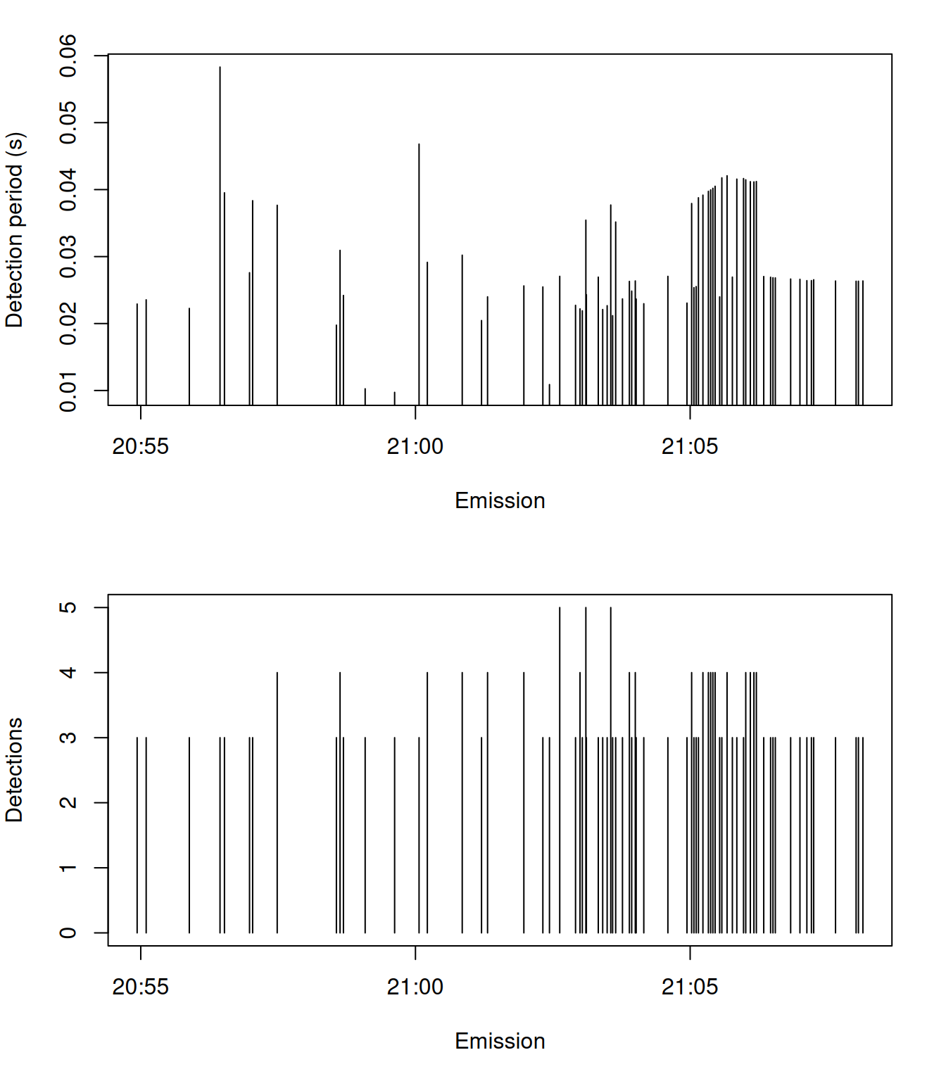
##              1        2            3         4            5   6
## 1   0.07564392      NaN   0.05880208       NaN   0.05273086 NaN
## 2          NaN      NaN   9.93697608  9.913433   9.93068606 NaN
## 3          NaN      NaN  57.04168208 57.019425  57.03442502 NaN
## 4          NaN 90.61658  90.57929508 90.558276          NaN NaN
## 5  95.43655372      NaN  95.41773508 95.397029          NaN NaN
## 6 122.81395998      NaN 122.79467308       NaN 122.78637113 NaN
##                  time
## 1 2021-05-08 20:54:56
## 2 2021-05-08 20:55:05
## 3 2021-05-08 20:55:53
## 4 2021-05-08 20:56:26
## 5 2021-05-08 20:56:31
## 6 2021-05-08 20:56:58
The following sections will deal with applying positioning models to these TOAMatrix objects.