2.3 Estimating clock offset

After correcting for clock drift, here’s what our sync-tag transmission latencies look like.

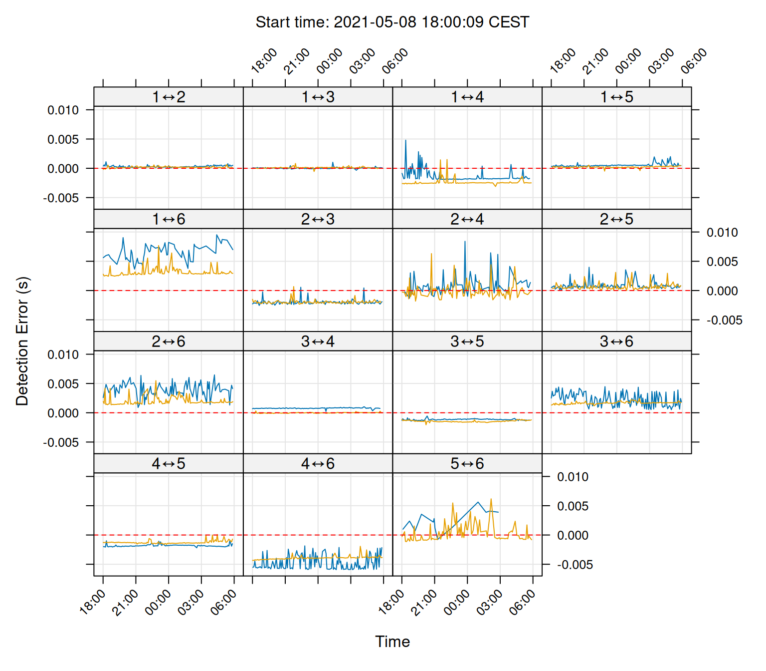
They no longer diverge over time, but some are far from the expected values (dashed red line). fit_clock_offsets() will automatically generate offset values for us to correct this.

This function will (by default) use the sync-tag data from all receivers in the array to calculate the offsets. This is done with a weighted least squares regression where the weights are taken from the inverse variance of mean latency measures for each receiver pair. That is to say, receiver pairs with highly variable sync-tag transmission latencies will contribute less to the estimated offset values.

Again, sync-tag detection error is treated as a mixture distribution (?ddetect).

# Fit clock offset values
clk_offsets <- fit_clock_offsets(sync_model, estimate_transmission_speed = T)
# View clock offset estimates
print(clk_offsets)

##  --- Kaltoa clock offset model
## Transmission speed
## 1444.83 m s⁻¹
## 
## Fitted offsets:
##   Receiver | Offset (s) | Std. Err.
##          1     -0.00047   3.37714     
##          3     -0.00039   3.62800     
##          4      0.00008   3.67073     
##          5     -0.00023   3.76820     
##          6     -0.00017   11.88684    
## 
## Residual mean latency (s):
## 1 -> 2:  0.00043
## 2 -> 1:  0.00009
## 1 -> 3:  0.00018
## 3 -> 1:  0.00002
## 1 -> 4: -0.00195
## 4 -> 1: -0.00222
## 1 -> 5:  0.00036
## 5 -> 1:  0.00045
## 1 -> 6:  0.00631
## 6 -> 1:  0.00319
## 2 -> 3: -0.00202
## 3 -> 2: -0.00199
## 2 -> 4:  0.00043
## 4 -> 2:  0.00012
## 2 -> 5:  0.00046
## 5 -> 2:  0.00087
## 2 -> 6:  0.00370
## 6 -> 2:  0.00217
## 3 -> 4:  0.00048
## 4 -> 3:  0.00036
## 3 -> 5: -0.00144
## 5 -> 3: -0.00114
## 3 -> 6:  0.00205
## 6 -> 3:  0.00192
## 4 -> 5: -0.00174
## 5 -> 4: -0.00135
## 4 -> 6: -0.00468
## 6 -> 4: -0.00401
## 5 -> 6:  0.00259
## 6 -> 5:  0.00025

# Save in KaltoaClockSync model
clock_offsets(sync_model) <- clk_offsets
# Plot disgnostics
plot(sync_model, type = 'error')

These results look much better now. Note how we also estimated the transmission speed here. The new transmission speed value will also be stored in our KaltoaClockSync object.

The bias for many receiver pairs has been reduced. However, the remaining bias is likely a result of incorrect receiver locations. The next section will cover how we can deal with poor receiver location data.