3.4 Population Monte Carlo (PMC-TOA)

Unfortunately, acoustically reflective features are often present where we do acoustic telemetry studies. In the case that large outliers resulting from transmission reflections are present, a more flexible positioning model is called for.

KaltoaPointPositioning solves positions using a form of adaptive importance sampling termed population Monte Carlo. Here, positions are solved according to the algorithm described in Campbell et al. (2025). The attractive feature of this algorithm is that positions can be solved quite fast with arbitrarily complex detection error distributions. Here, we’ll specify an error distribution that takes into account large outliers resulting from reflected tag transmissions.

First, we need to specify our detection error distribution. kaltoa stores this in a KaltoaObservationModel object.

# Make observation model
c = 1420# (m/s) Speed of tag transmission
max_trns_lat <- 500 / c# (s) Max transmission latency 
obs_sigma <- 0.002# (s) Standard deviation for direct detection distribution
obs_beta <- 128# Shape parameter for reflected detection distribution
obsv_model <- KaltoaObservation(
  type = "mixed", sigma = obs_sigma, beta = obs_beta, 
  max_transmission_latency = max_trns_lat)

# Show observation model
print(obsv_model)
plot(obsv_model)
plot(obsv_model, xlim = c(-0.01, 0.03), ylim = c(0, 10))

## KaltoaObservationModel
## Type: mixed
## Maximum transmission latency: 0.4 s
## Parameters: sigma: 0.002, beta: 128.0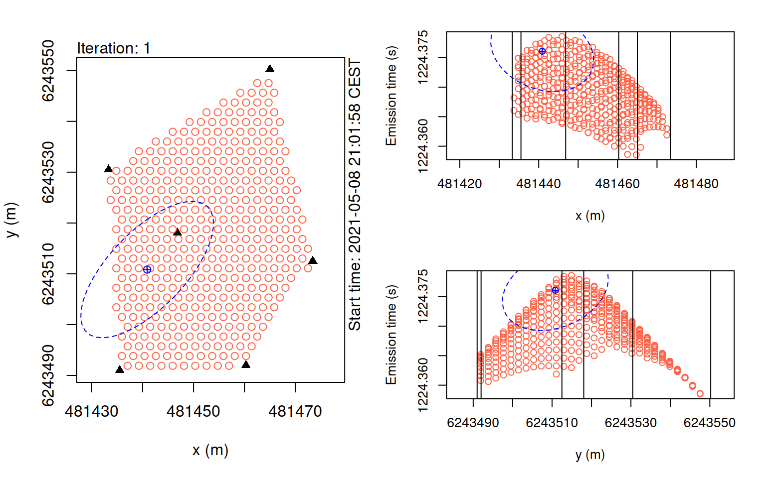

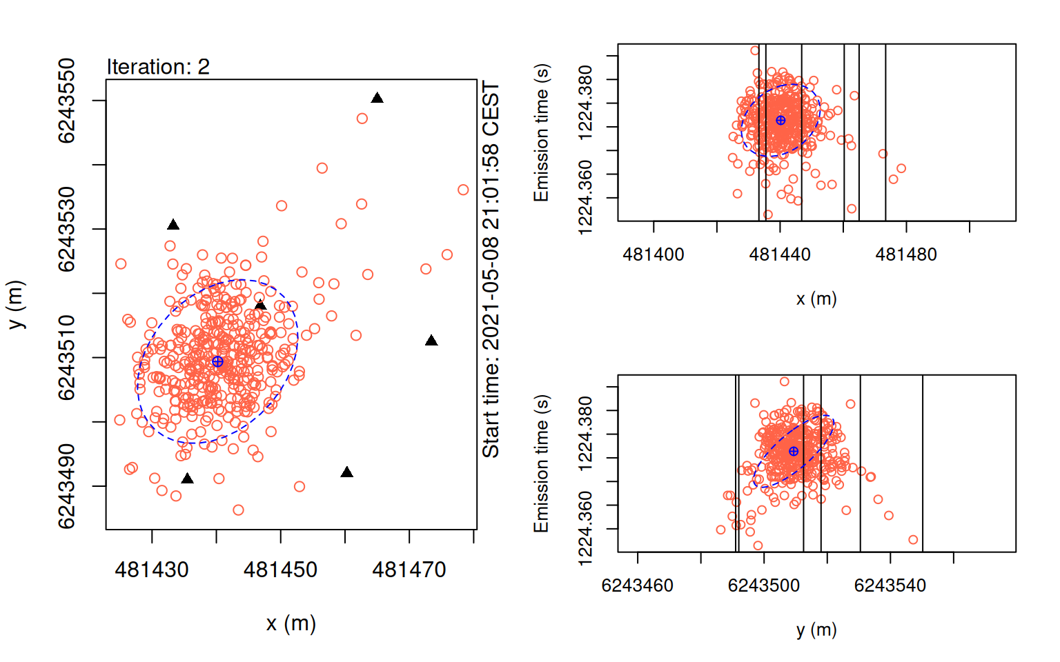
First, we’ll position a single emission. From here, we can verify our model has been parameterized well by inspecting diagnostic plots.

# Apply positioning model
points_pmc <- KaltoaPointPositioning(toa_comp[112], observation_model = obsv_model, 
  iter = 4, quietly = T, n_particles = 400)

# Plot particle convergence
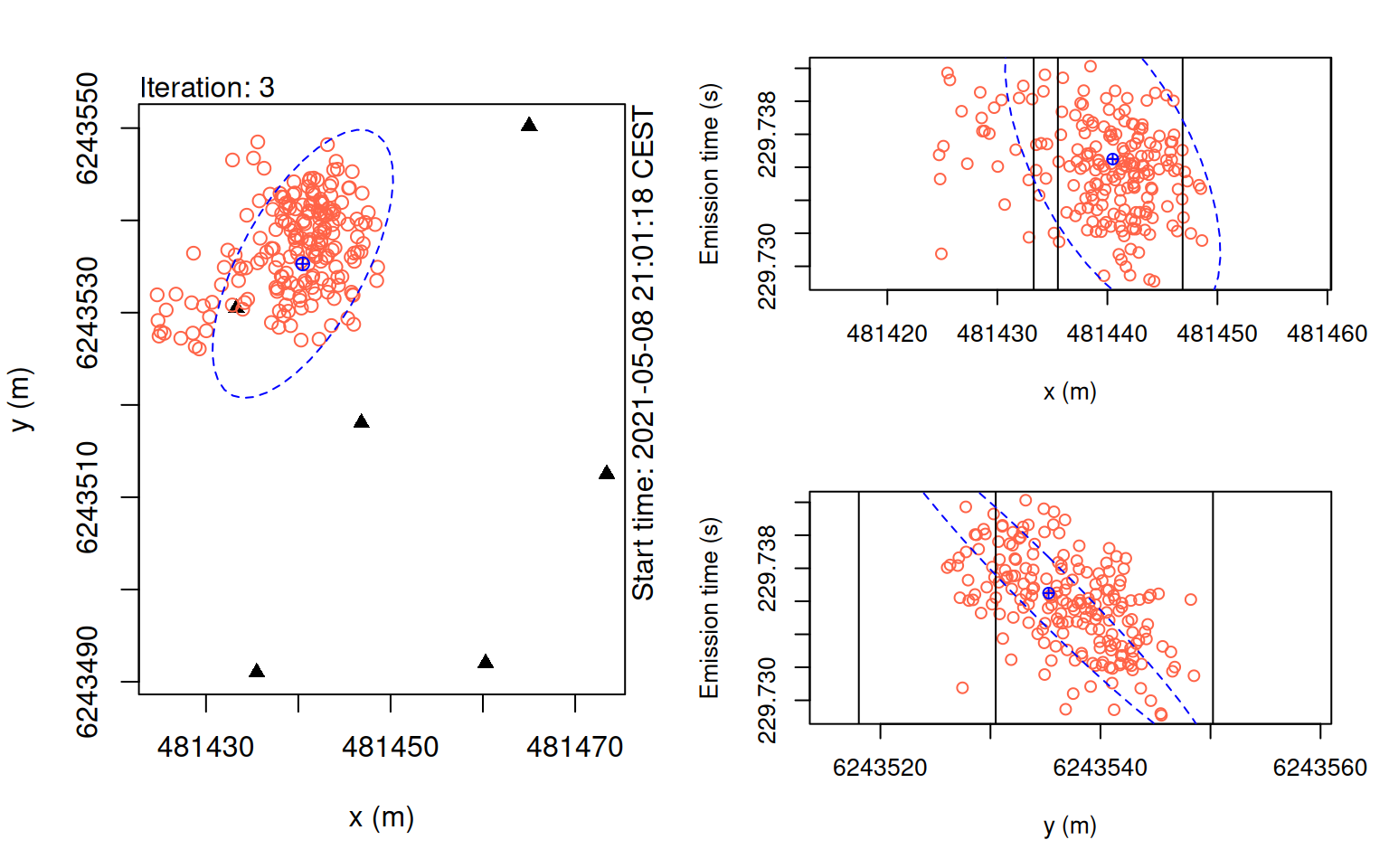
plot(points_pmc, iter = 1)
plot(points_pmc, iter = 2)
plot(points_pmc, iter = 3)
plot(points_pmc, iter = 4)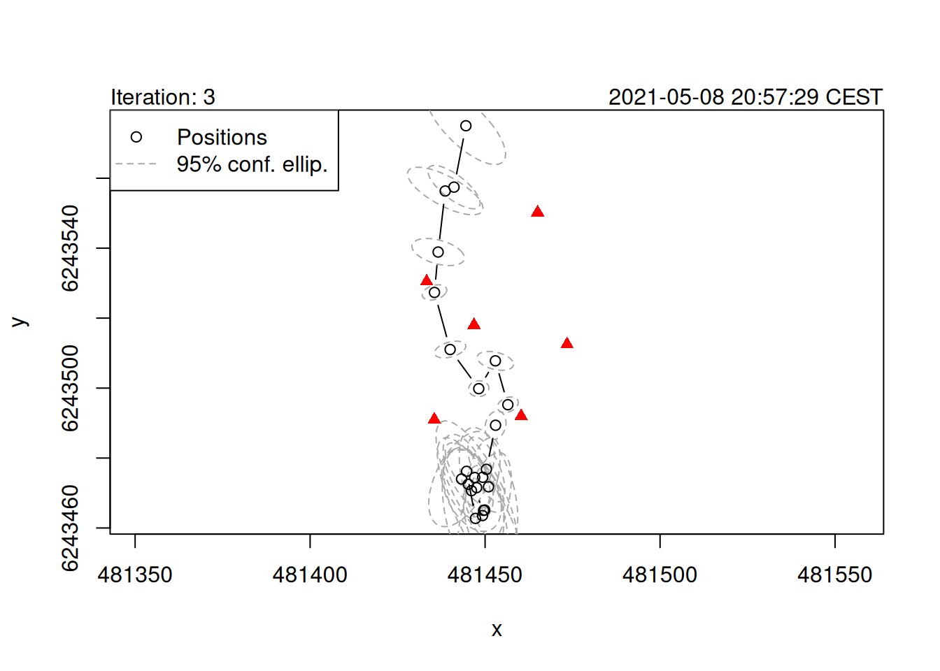

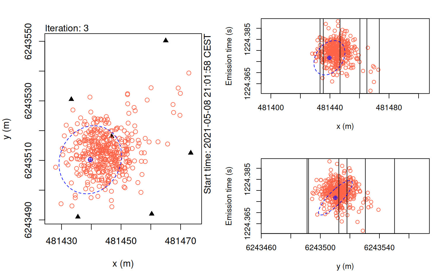
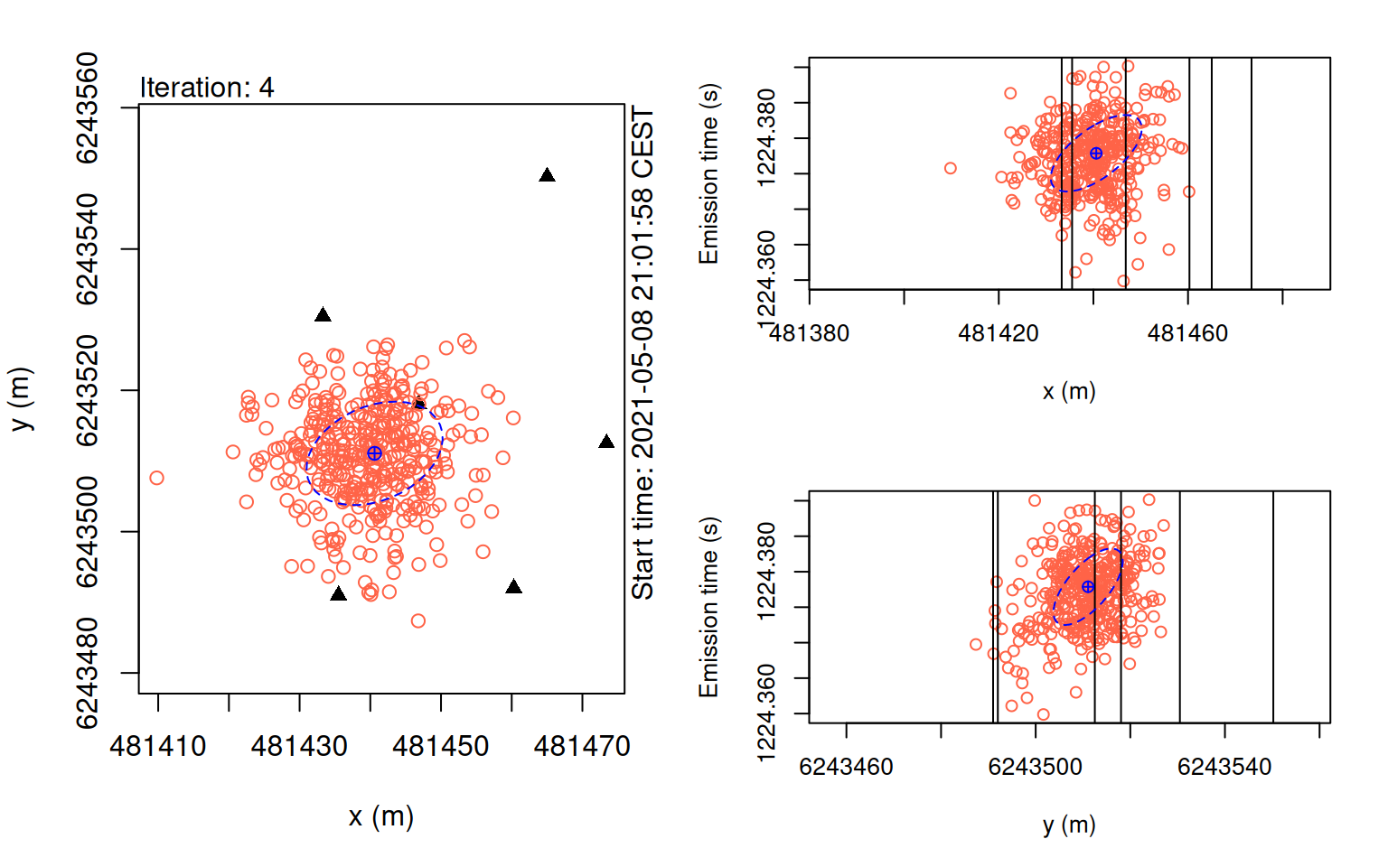
In these plots, we want to check that our particles gradually converging towards a central estimate. If the KaltoaObservationModel’s sigma, or pertubation_sigma is set too small, the particles may get ‘stuck’ in locations which can cause issues for convergence. Additionally, too few particles can also result in this problem.

The key to using this model is striking a balance between processing time and stability of the algorithm. In general, we suggest setting one more iteration than appears necessary and experimenting for stable values for n_particles.

Now we’re happy with our model parameters, let’s run the positioning on the whole data set.

points_pmc <- KaltoaPointPositioning(
  toa = subset(toa_comp, detections >= 4 & period < 0.1),
  observation_model = obsv_model, 
  iter = 4, quietly = T, n_particles = 400)
plot(points_pmc)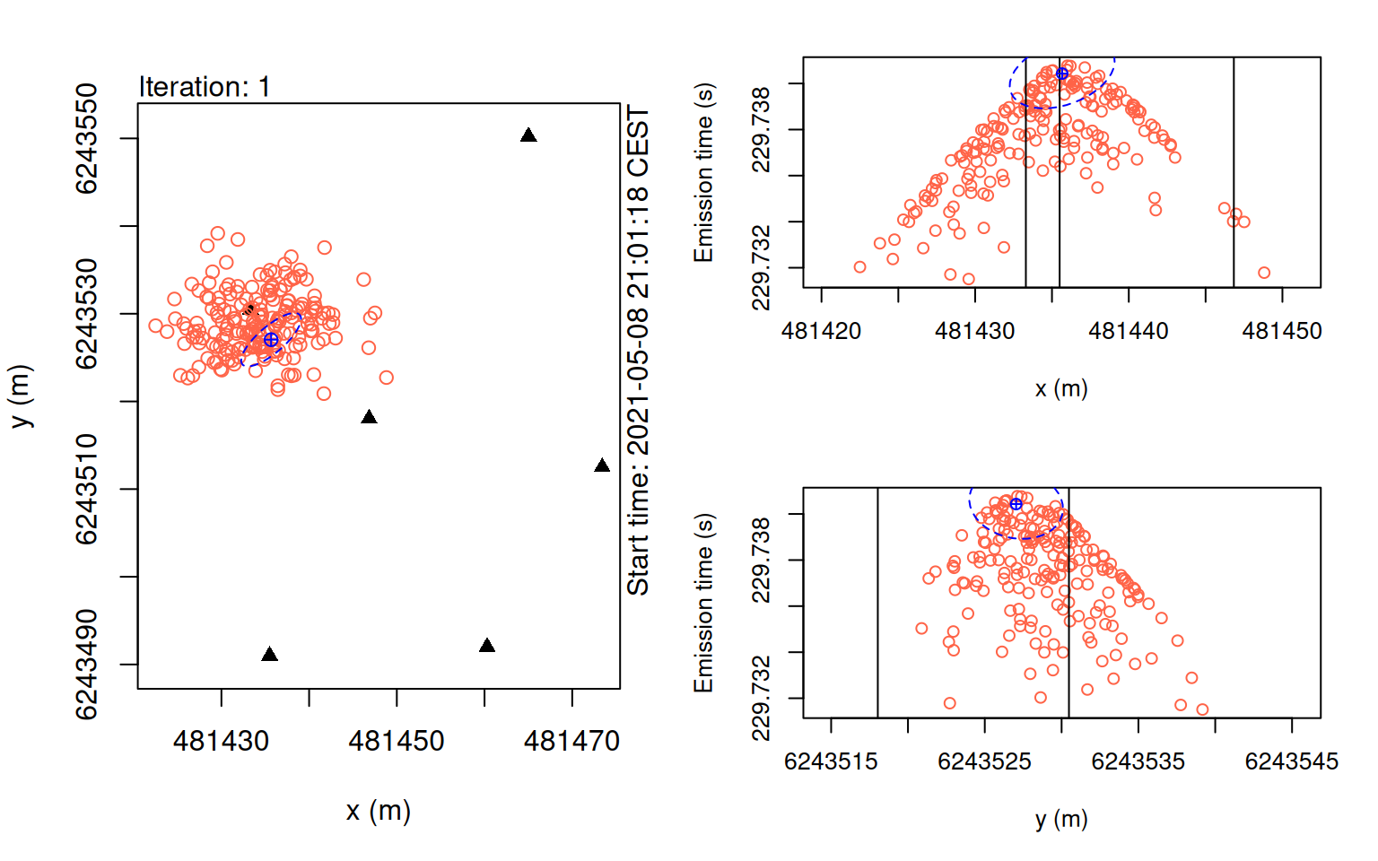

Here, we used a direct detection standard deviation of 0.002 (see print(obsv_model)). Note that earlier we decided that a value of 0.0008 is likely more appropriate for this data set.

When using precise detection error distributions, PMC-TOA requires either (a) more particles, or (b) better initial positions to avoid sample impovrishment and converge in a stable manner.

To fit the ideal detection error value of 0.0008, we can refit the PMC-TOA algorithm using the estimated positions from our previous run. This second run of PMC-TOA has much higher quality initial positions as they are selected from a smaller, more important region of the study area. As a result, we can refit more precise detection error distributions with a small number of particles.

# Create a precise observation model
# This has a small standard deviation for direct detection error
obsv_model_2 <- KaltoaObservation(
  type = "mixed", sigma = sigma_det, beta = obs_beta, 
  max_transmission_latency = max_trns_lat)
print(obsv_model_2)

## KaltoaObservationModel
## Type: mixed
## Maximum transmission latency: 0.4 s
## Parameters: sigma: 8e-04, beta: 128.0

# Refit the PMC-TOA algorithm with a lower number of particles
points_pmc_2 <- KaltoaPointPositioning(
  toa = subset(toa_comp, detections >= 4 & period < 0.1), 
  observation_model = obsv_model_2, 
  iter = 3, quietly = T, n_particles = 200,
  init_positions = points_pmc)
plot(points_pmc_2)

# Visualize convergence
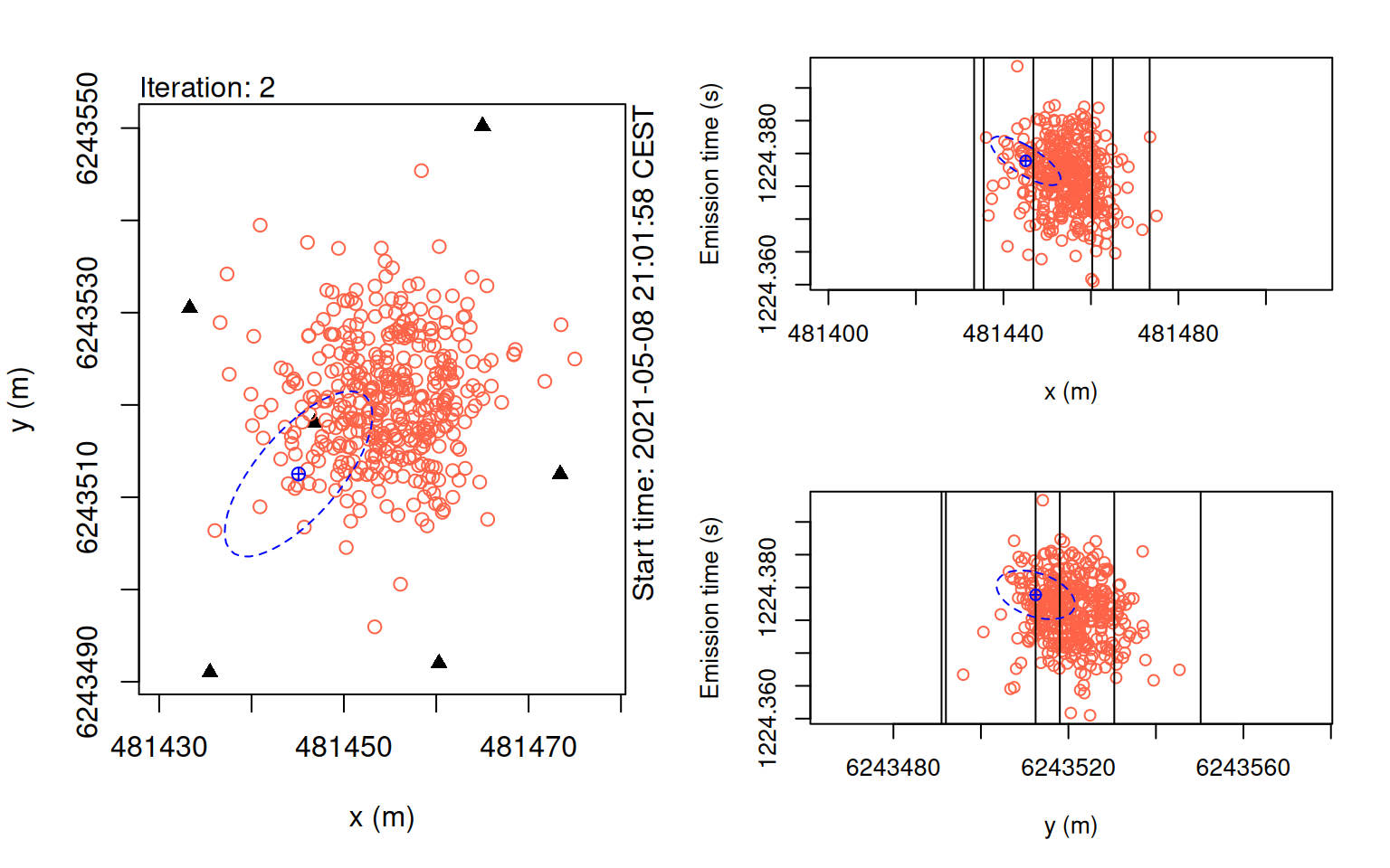
plot(points_pmc_2, i = 5, iter = 1)
plot(points_pmc_2, i = 5, iter = 2)
plot(points_pmc_2, i = 5, iter = 3)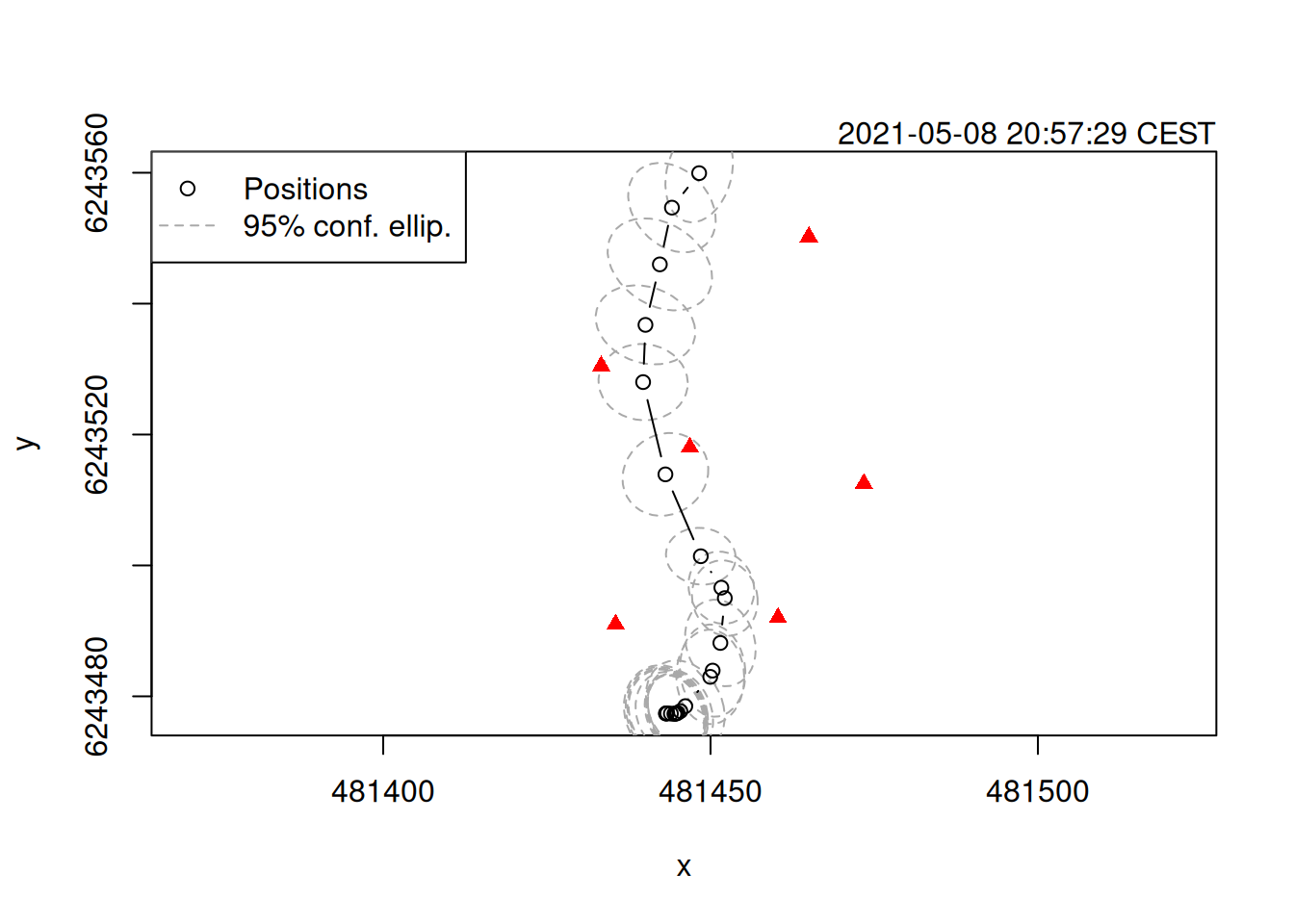

In the above example, if we tried to fit this precise KaltoaObservationModel with the default initial positions (a uniform sample from the whole study area), there would be a high risk of sample impoverishment and the resulting estimates would be unstable.

• Campbell, J. A., Shry, S. J., Lundberg, P., Calles, O., Hoelker, F. 2025. A population Monte Carlo model for underwater acoustic telemetry positioning in reflective environments. Methods Ecology and Evolution. 16(4). 775-785.