3.6 Applying corrections

Now that our sync-tag diagnostic plots look quite good, we can apply the corrections to our Detectionslist object.

# Create corrected detections dataset
detlst_corr <- synchronize(exdata_clocksync, sync_model)

# Plot sync-tag diagnostics
sync_lat <- SyncTagLatency(detlst_corr)
c <- transmission_speed(sync_model)
plot(sync_lat, transmission_speed = c)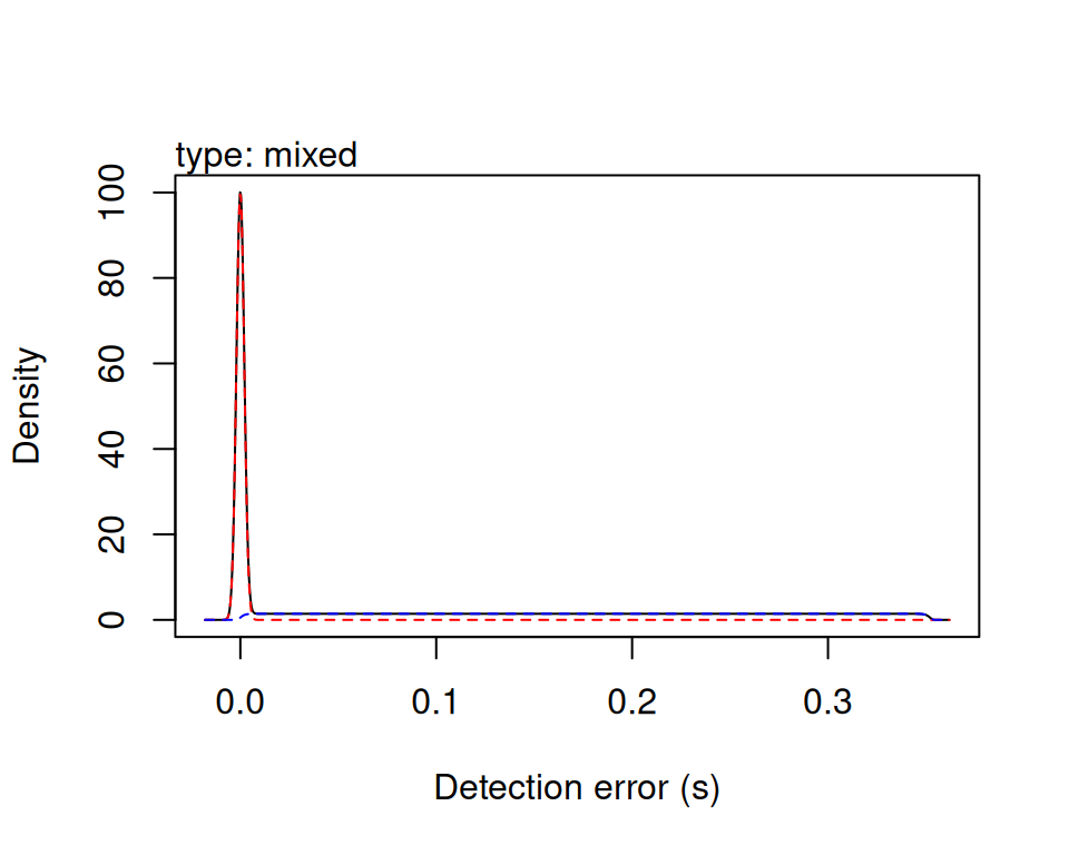

plot(sync_lat, transmission_speed = c, type = 'error')

plot(sync_lat, transmission_speed = c, type = 'error', hist = T, nint = 20)

We now have sync-tag transmission values that match well with our expectations. We can now apply telemetry positioning models to this data set.

Lastly, it can be useful to use the sync-tags to take empirical measures of your detection error. This detection error distribution can be later used in telemetry positioning models.

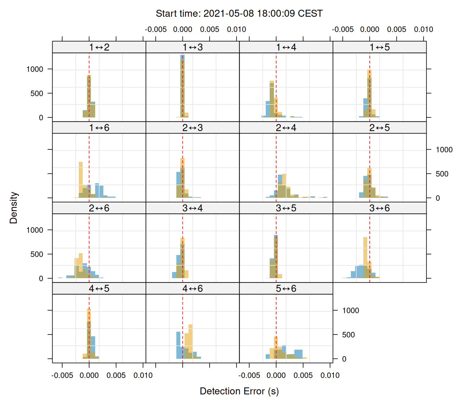
This can be easily done with the detection_error function. Below we’ll (i) extract the sync-tag detection error values, then (ii) fit a mixed detection error distribution (ddetect) to those values.

# Extract detection error for SyncTagLatency object
det_err <-  detection_error(sync_lat, transmission_speed = c)
head(det_err); tail(det_err)

##   pair path detection_error
## 1  1↔2  1⟶2    0.0004174217
## 2  1↔2  1⟶2    0.0005618233
## 3  1↔2  1⟶2    0.0003061578
## 4  1↔2  1⟶2    0.0009987495
## 5  1↔2  1⟶2    0.0002098794
## 6  1↔2  1⟶2    0.0001690051

##      pair path detection_error
## 3171  5↔6  6⟶5    0.0001362564
## 3172  5↔6  6⟶5    0.0026961492
## 3173  5↔6  6⟶5    0.0004466531
## 3174  5↔6  6⟶5    0.0009695442
## 3175  5↔6  6⟶5    0.0007224886
## 3176  5↔6  6⟶5    0.0006194381

# Get histogram of empirical detection error distribution
hist <- hist(det_err$detection_error, plot = F, breaks = 50)

# Set phi to double the largest detection error value
phi <- max(det_err$detection_error, na.rm = T) * 2

# Fit the sigma parameter
res <- optim(
  par = c(sigma = 0.1), method = "Brent",
  lower = 0, upper = 1,
  fn = \(par){
    # Get negative log likelihood
    ret <- -ddetect(
      x = na.omit(det_err$detection_error), 
      sigma = par[1], phi = phi, 
      log = T) |> sum()
  })
sigma <- res$par
message(sprintf("Fitted detection error \u03c3: %.5f s", sigma))

## Fitted detection error σ: 0.00088 s

# Get fitted detection error distribution
x_rng <- range(det_err$detection_error, na.rm = T)
x <- seq(x_rng[1], x_rng[2], by = 1e-4)
y <- ddetect(x = x, sigma = sigma, phi = phi)

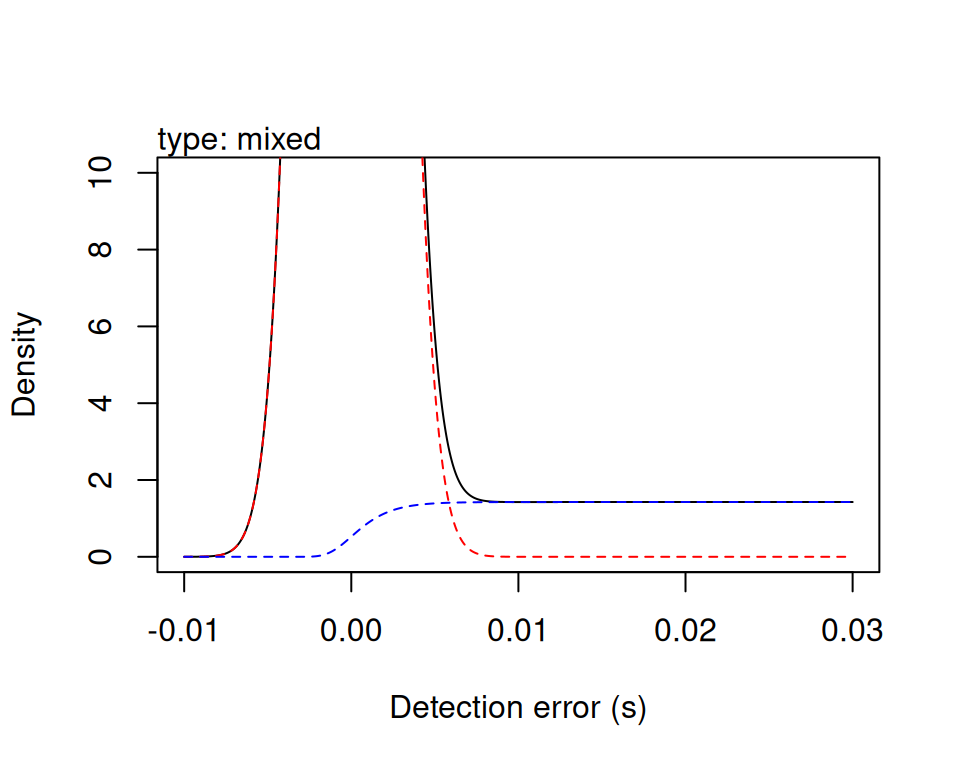
# Plot fitted vs. empirical detection error
ymax <- max(c(hist$density, y))
plot(NULL, xlim = range(x_rng), ylim = c(0, ymax),
  ylab = "Density", xlab = "Detection error (s)")
lines(hist$mids, hist$density, type = "h", col = "steelblue")
lines(x,y, lty = 2, col = "tomato")
legend(x = "topright", 
  legend = c("Measured detection error", "Fitted detection error"), 
  col = c("steelblue", "tomato"), lty = c(1,2))

The above values for phi and sigma can be used with the KaltoaPointPositioning function.