3.2 Measuring detection error

Positioning models in kaltoa require the detection error to be measured beforehand. The SyncTagLatency objects we used earlier to visualize our clock corrections can be used for this purpose.

# Plot detection error
plot(SyncTagLatency(exdata_positioning), type = "error",
  transmission_speed = 1420, layout = c(4,4))

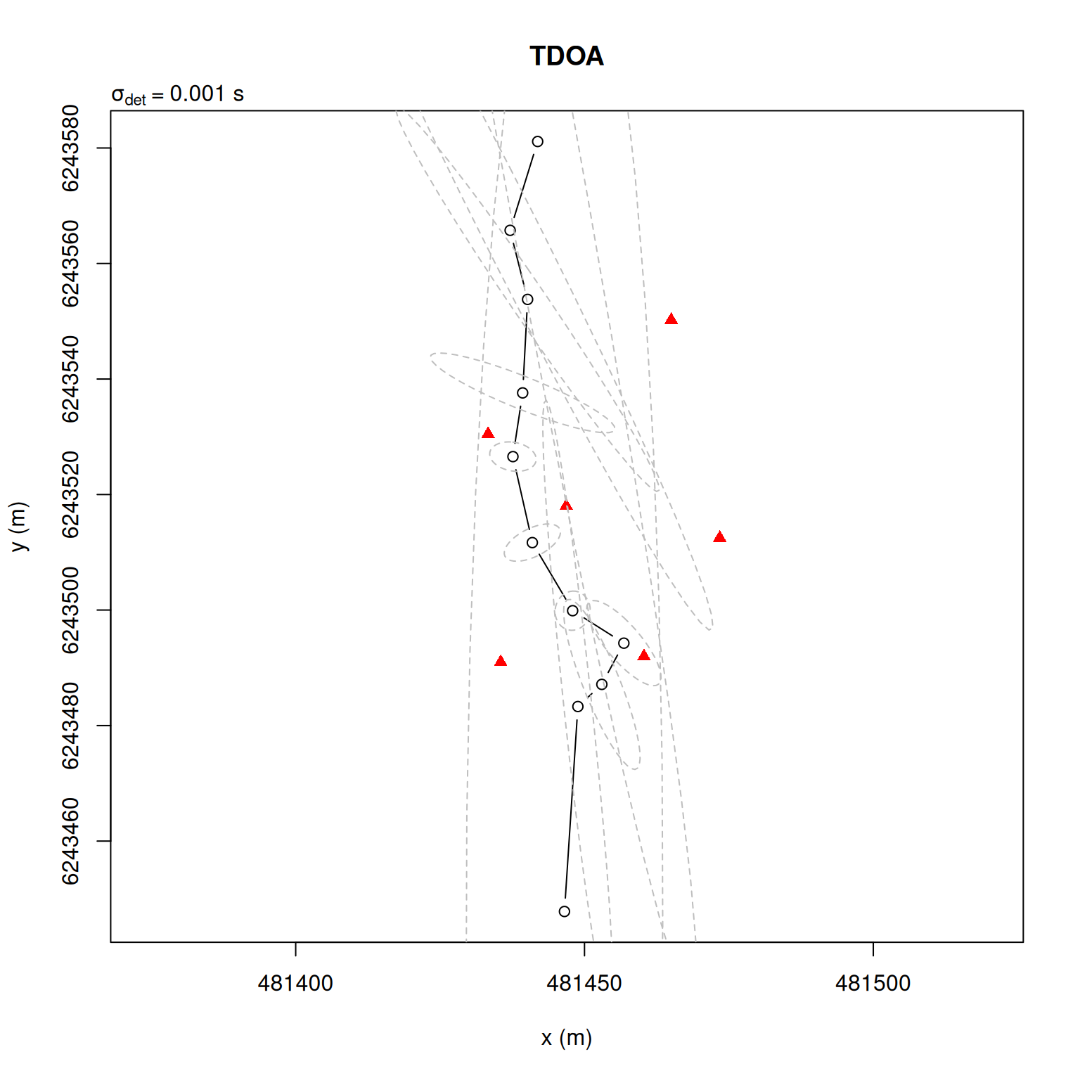
A simple approach is to draw the desired direct detection error distribution and overlay it on the SyncTagLatency histogram plot.

# Direct detection error
sigma_det <- 0.0008
  
# Draw a Gaussian direct error distribution
df_error <- data.frame(error = seq(-0.004, 0.004, length.out = 100))
df_error$dens <- dnorm(df_error$error, sd = sigma_det)

# Overlay detection error distribution on histograms of sync-tag detection errors
plot(SyncTagLatency(exdata_positioning), type = "error", 
  hist = T, transmission_speed = 1420, nint = 20, 
  subset = abs(error) < 0.004,
  layout = c(4,4)) + 
  latticeExtra::as.layer(xyplot(
    dens ~ error, data = df_error, type = 'l'))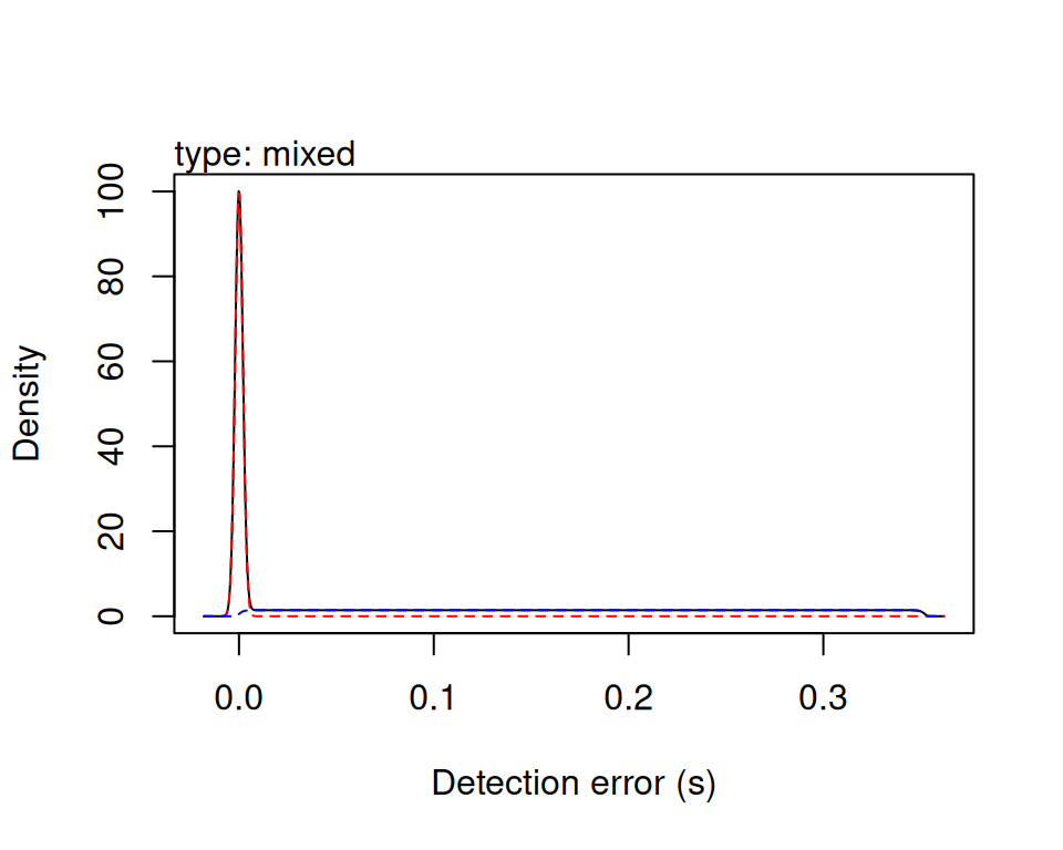

Here, we’ve chosen sigma_det so it broadly captures the sync-tag detections which we judge to be resulting from direct detections. We’re ignoring large positive outliers here, as these are likely due to reflections and can be captured by a mixture detection error distribution (ddetect).

So long as you don’t have large negative outliers (i.e. detection occurring before they are expected), we’re in good hands here.