3.2 Estimating clock drift
For correcting clock drift, we need to first provide some reasonably good guesses of the true drift values.
permute_clock_drift() can take care of this.
This function takes a brute force approach that permutes across a series of plausible drift values to see how closely the sync-tag detections and emissions line up between a receiver pair.
There are two available methods for measuring how well the emissions and detections line up and both have their particular use case.
- xcorr: Emissions and detections are represented as Gaussian kernels drawn along two time-series. Cross correlation is applied and the most likely drift value is the one which results in the most overlap between these emission and detection kernels (i.e. the highest cross-correlation score).
- likelihood: Emissions are arranged in a time-series and a mixed detection error distribution is drawn over each emission event. Detections are then sampled from this and the joint likelihood that any detection originated from any emission is returned for each drift value. The drift value resulting in the maximum likelihood is chosen.
The xcorr method is preferred if some emission events may be missing from the dataset. However, if there are more reflections than direct detections between the receiver pair, this method risks using the late-arriving reflected sync-tag transmissions to select the drift values.
Conversely, the likelihood method directly accounts for the presence of reflections by treating the detection error as a mixed distribution (see ?ddetect()).
This method assumes that all detection events have a corresponding emission event.
If a few emission events are missing from the dataset, this can cause low likelihood scores.
Both methods are coded by treating the underlying math as convolution operations in the Fourier domain, hence they run extremely fast for the amount of data they process.
These work well for getting values on the scale of, say, 0.1 second resolution.
For each clock_time, we’ll check possible drift values within a 1 hour-period
int_drft_xcor <- permute_clock_drift(
  sync_model,
  method = "xcorr",# Evaluate emission/detection alignment with cross-correlation
  clock_resolution = 0.1,# (s) Resolution of the emission/detection time-series
  clock_window = 60*60*1,# (s) Length of window to estimate drift values from
  sigma = 0.1*5,# (s) Width of Gaussian kernel
  quiet = T)
print(int_drft_xcor)
## Clock drift permutation values
## Receiver pair: 3 ⟷ 1
## Drift (s) xcorr
## 2021-05-08 18:00:00 0.4 1.35
## 2021-05-08 19:00:00 0.4 1.39
## 2021-05-08 20:00:00 0.4 1.18
## 2021-05-08 21:00:00 0.4 1.27
## 2021-05-08 22:00:00 0.4 1.38
## 2021-05-08 23:00:00 0.4 1.39
## 2021-05-09 00:00:00 0.4 1.34
## 2021-05-09 01:00:00 0.5 1.18
## 2021-05-09 02:00:00 0.5 1.21
## 2021-05-09 03:00:00 0.5 1.18
## 2021-05-09 04:00:00 0.5 1.17
## 2021-05-09 05:00:00 0.5 1.21
## 2021-05-09 06:00:00 0.5 1.14
##
## Receiver pair: 3 ⟷ 2
## Drift (s) xcorr
## 2021-05-08 18:00:00 33.20000 1.41
## 2021-05-08 19:00:00 33.30000 1.35
## 2021-05-08 20:00:00 33.30000 1.12
## 2021-05-08 21:00:00 33.40000 1.30
## 2021-05-08 22:00:00 33.60000 1.25
## 2021-05-08 23:00:00 33.60000 1.24
## 2021-05-09 00:00:00 33.70000 1.28
## 2021-05-09 01:00:00 33.80000 1.20
## 2021-05-09 02:00:00 33.90000 1.19
## 2021-05-09 03:00:00 34.00000 1.24
## 2021-05-09 04:00:00 34.00000 1.23
## 2021-05-09 05:00:00 34.10000 1.19
## 2021-05-09 06:00:00 34.21061 NaN
##
## Receiver pair: 3 ⟷ 4
## Drift (s) xcorr
## 2021-05-08 18:00:00 34.60000 1.42
## 2021-05-08 19:00:00 34.70000 1.38
## 2021-05-08 20:00:00 34.70000 1.16
## 2021-05-08 21:00:00 34.80000 1.33
## 2021-05-08 22:00:00 34.90000 1.27
## 2021-05-08 23:00:00 35.00000 1.28
## 2021-05-09 00:00:00 35.10000 1.26
## 2021-05-09 01:00:00 35.20000 1.12
## 2021-05-09 02:00:00 35.30000 1.33
## 2021-05-09 03:00:00 35.40000 1.23
## 2021-05-09 04:00:00 35.50000 1.22
## 2021-05-09 05:00:00 35.50000 0.91
## 2021-05-09 06:00:00 35.63788 NaN
##
## Receiver pair: 3 ⟷ 5
## Drift (s) xcorr
## 2021-05-08 18:00:00 30.1 1.41
## 2021-05-08 19:00:00 30.2 1.38
## 2021-05-08 20:00:00 30.2 1.21
## 2021-05-08 21:00:00 30.3 1.23
## 2021-05-08 22:00:00 30.4 1.28
## 2021-05-08 23:00:00 30.5 1.20
## 2021-05-09 00:00:00 30.5 1.19
## 2021-05-09 01:00:00 30.6 1.04
## 2021-05-09 02:00:00 30.7 1.27
## 2021-05-09 03:00:00 30.8 1.33
## 2021-05-09 04:00:00 30.8 1.37
## 2021-05-09 05:00:00 30.9 1.09
## 2021-05-09 06:00:00 30.9 0.97
##
## Receiver pair: 4 ⟷ 6
## Drift (s) xcorr
## 2021-05-08 18:00:00 4.3 1.31
## 2021-05-08 19:00:00 4.3 1.37
## 2021-05-08 20:00:00 4.3 1.28
## 2021-05-08 21:00:00 4.4 1.35
## 2021-05-08 22:00:00 4.4 1.29
## 2021-05-08 23:00:00 4.4 1.31
## 2021-05-09 00:00:00 4.4 1.34
## 2021-05-09 01:00:00 4.4 1.23
## 2021-05-09 02:00:00 4.4 1.28
## 2021-05-09 03:00:00 4.4 1.34
## 2021-05-09 04:00:00 4.4 1.20
## 2021-05-09 05:00:00 4.4 1.45
## 2021-05-09 06:00:00 4.5 1.20When using this method, be sure to select a sufficiently large Gaussian kernel based on the amount of drift you expect in your receiver array.
In other words, how much drift you expect to occur within the clock_window period.
Wider kernels will return higher cross correlation scores when an emission is “almost, but not quite” aligned with a detection event.
Each drift estimate is returned along with its cross correlation score, xcorr.
These will range from 0-1, with higher values indicating better fitting drift values.
Next we can plot out our estimated drift values.
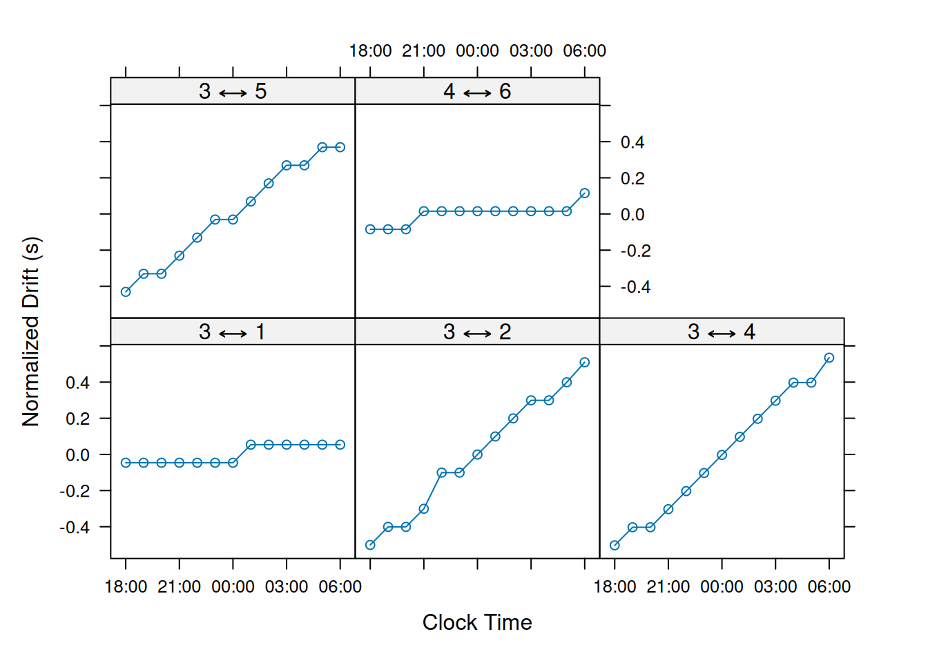
The y-axis shows the drift rate. That is, the change in the drift values normalized by the period between the clock times—seconds of additional drift per hour of time.
Let’s also do an example of using the likelihood method.
Here, rather than specifying the scale of our Gaussian kernel, we provide the parameters of a mixed detection error distribution, sigma_det, phi, and beta.
sigma_det is the standard deviation of the Gaussian which captures direct detections while phi is the upper limit of the approximate uniform distribution that captures late arriving reflections.
phi is more-less the maximum possible detection error that a late-arriving reflection can result in.
int_drft_lik <- permute_clock_drift(
  sync_model,
  method = "like",# Evaluate emission/detection alignment with cross-correlation
  clock_resolution = 0.1,# (s) Resolution of the emission/detection time-series
  clock_window = 60*60*1,# (s) Length of window to estimate drift values from
  sigma_det = 0.1,# (s) Standard deviation of direct detection error
  phi = 0.5,# (s) Maximum additional latency from reflected detections
  quiet = T)
print(int_drft_lik)
## Clock drift permutation values
## Receiver pair: 3 ⟷ 1
## Drift (s) Rel. logLik.
## 2021-05-08 18:00:00 0.4 -5.68
## 2021-05-08 19:00:00 0.4 -3.90
## 2021-05-08 20:00:00 0.4 -6.89
## 2021-05-08 21:00:00 0.4 -6.39
## 2021-05-08 22:00:00 0.4 -4.16
## 2021-05-08 23:00:00 0.4 -5.23
## 2021-05-09 00:00:00 0.4 -5.84
## 2021-05-09 01:00:00 0.4 -5.53
## 2021-05-09 02:00:00 0.4 -6.57
## 2021-05-09 03:00:00 0.5 -6.03
## 2021-05-09 04:00:00 0.5 -5.28
## 2021-05-09 05:00:00 0.5 -7.07
## 2021-05-09 06:00:00 0.5 -4.15
##
## Receiver pair: 3 ⟷ 2
## Drift (s) Rel. logLik.
## 2021-05-08 18:00:00 33.2 -2.24
## 2021-05-08 19:00:00 33.3 -4.50
## 2021-05-08 20:00:00 33.4 -7.55
## 2021-05-08 21:00:00 33.4 -6.28
## 2021-05-08 22:00:00 33.5 -7.63
## 2021-05-08 23:00:00 33.6 -6.30
## 2021-05-09 00:00:00 33.7 -5.98
## 2021-05-09 01:00:00 33.8 -3.00
## 2021-05-09 02:00:00 33.8 -5.52
## 2021-05-09 03:00:00 33.9 -6.64
## 2021-05-09 04:00:00 34.0 -5.26
## 2021-05-09 05:00:00 34.1 -8.40
## 2021-05-09 06:00:00 34.2 -2.50
##
## Receiver pair: 3 ⟷ 4
## Drift (s) Rel. logLik.
## 2021-05-08 18:00:00 34.6 -5.09
## 2021-05-08 19:00:00 34.7 -4.34
## 2021-05-08 20:00:00 34.7 -7.24
## 2021-05-08 21:00:00 34.8 -4.83
## 2021-05-08 22:00:00 34.9 -6.34
## 2021-05-08 23:00:00 35.0 -6.03
## 2021-05-09 00:00:00 35.1 -4.08
## 2021-05-09 01:00:00 35.2 -7.56
## 2021-05-09 02:00:00 35.2 -2.85
## 2021-05-09 03:00:00 35.3 -3.85
## 2021-05-09 04:00:00 35.4 -5.76
## 2021-05-09 05:00:00 35.5 -9.35
## 2021-05-09 06:00:00 35.6 -2.16
##
## Receiver pair: 3 ⟷ 5
## Drift (s) Rel. logLik.
## 2021-05-08 18:00:00 30.1 -2.26
## 2021-05-08 19:00:00 30.2 -4.14
## 2021-05-08 20:00:00 30.2 -6.88
## 2021-05-08 21:00:00 30.3 -6.75
## 2021-05-08 22:00:00 30.4 -5.92
## 2021-05-08 23:00:00 30.5 -6.96
## 2021-05-09 00:00:00 30.5 -5.64
## 2021-05-09 01:00:00 30.6 -8.23
## 2021-05-09 02:00:00 30.7 -4.73
## 2021-05-09 03:00:00 30.8 -4.64
## 2021-05-09 04:00:00 30.9 -3.14
## 2021-05-09 05:00:00 30.9 -9.47
## 2021-05-09 06:00:00 31.0 -3.33
##
## Receiver pair: 4 ⟷ 6
## Drift (s) Rel. logLik.
## 2021-05-08 18:00:00 4.3 -7.78
## 2021-05-08 19:00:00 4.3 -5.40
## 2021-05-08 20:00:00 4.3 -6.22
## 2021-05-08 21:00:00 4.3 -4.46
## 2021-05-08 22:00:00 4.3 -5.11
## 2021-05-08 23:00:00 4.4 -6.00
## 2021-05-09 00:00:00 4.4 -3.12
## 2021-05-09 01:00:00 4.4 -6.68
## 2021-05-09 02:00:00 4.4 -3.86
## 2021-05-09 03:00:00 4.4 -1.34
## 2021-05-09 04:00:00 4.4 -7.90
## 2021-05-09 05:00:00 4.4 -3.80
## 2021-05-09 06:00:00 4.4 -7.32
Here, the quality of the drift estimates are given by a relative likelihood score. This is the maximum possible log likelihood subtracted the measured log likelihood, then divided by the number of detection events. If all detection events fall along the peaks of the error distributions, the relative likelihood score will be 0.
Now we’ll store our initial drift values in our KaltoaClockSync object.
# Save drift values to KaltoaClockSync model
clock_drift(sync_model) <- int_drft_lik
# Plot sync-tag diagnostics
plot(sync_model, layout = c(4,4))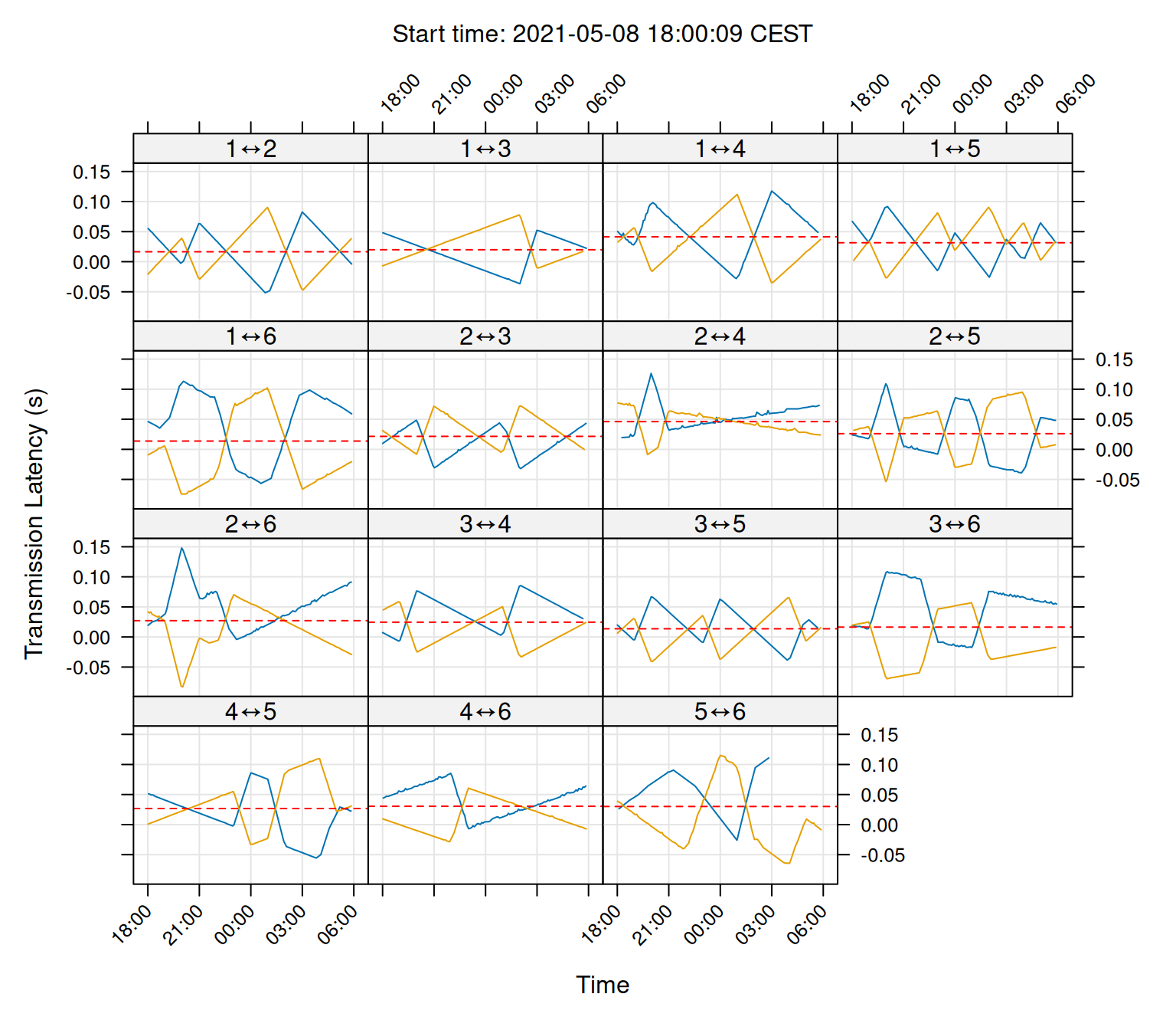
As you can see in the plot, our clocks are roughly corrected within a 0.1 second resolution. For fine-scale positioning, we need to refine this further.
fit_clock_drift will automatically refine these clock drift values.
For each receiver pair, the clock drift is treated a a Gaussian random walk along some linear trend line.
The drift values are fitted as random effects in the R package TMB and the detection error is treated as a mixture distribution (see ?ddetect).
This function can provide extremely high resolution drift values.
However, for the model to fit, it requires quite good starting values.
We suggest using permute_clock_drift to get drift values with at least a 0.1 second resolution before applying fit_clock_drift.
fit_drft_1 <- fit_clock_drift(
  sync_model, quiet = T,
  sigma_det = 0.01,# (s) Initial value for the direct detection error
  fix_sigma_det = T# Do not fit the direct detection error parameter
  )
print(fit_drft_1)
## --- Kaltoa receiver drift model
## Detection σ (ms) Drift (ms h⁻¹) Drift σ (ms h⁻¹)
## 3 ⟷ 1 10 10.605 0.026584
## 3 ⟷ 2 10 80.326 0.14279
## 3 ⟷ 4 10 84.844 0.059035
## 3 ⟷ 5 10 73.9 0.059727
## 4 ⟷ 6 10 9.876 0.007577
## Trns. lat. (ms)
## 3 ⟷ 1 20.242
## 3 ⟷ 2 20.297
## 3 ⟷ 4 25.824
## 3 ⟷ 5 12.682
## 4 ⟷ 6 26.767
##
## Drift values
## 3 ⟷ 1 3 ⟷ 2 3 ⟷ 4 3 ⟷ 5 4 ⟷ 6
## 2021-05-08 18:00:00 0.37248 33.211 34.582 30.108 4.3173
## 2021-05-08 19:00:00 0.38309 33.291 34.667 30.181 4.3272
## 2021-05-08 20:00:00 0.39370 33.372 34.752 30.255 4.3371
## 2021-05-08 21:00:00 0.40430 33.452 34.837 30.329 4.3470
## 2021-05-08 22:00:00 0.41491 33.532 34.921 30.403 4.3568
## 2021-05-08 23:00:00 0.42551 33.613 35.006 30.477 4.3667
## 2021-05-09 00:00:00 0.43612 33.693 35.091 30.551 4.3766
## 2021-05-09 01:00:00 0.44672 33.773 35.176 30.625 4.3865
## 2021-05-09 02:00:00 0.45733 33.854 35.261 30.699 4.3963
## 2021-05-09 03:00:00 0.46793 33.934 35.346 30.773 4.4062
## 2021-05-09 04:00:00 0.47854 34.014 35.430 30.847 4.4161
## 2021-05-09 05:00:00 0.48914 34.095 35.515 30.920 4.4260
## 2021-05-09 06:00:00 0.49975 34.175 35.600 30.994 4.4358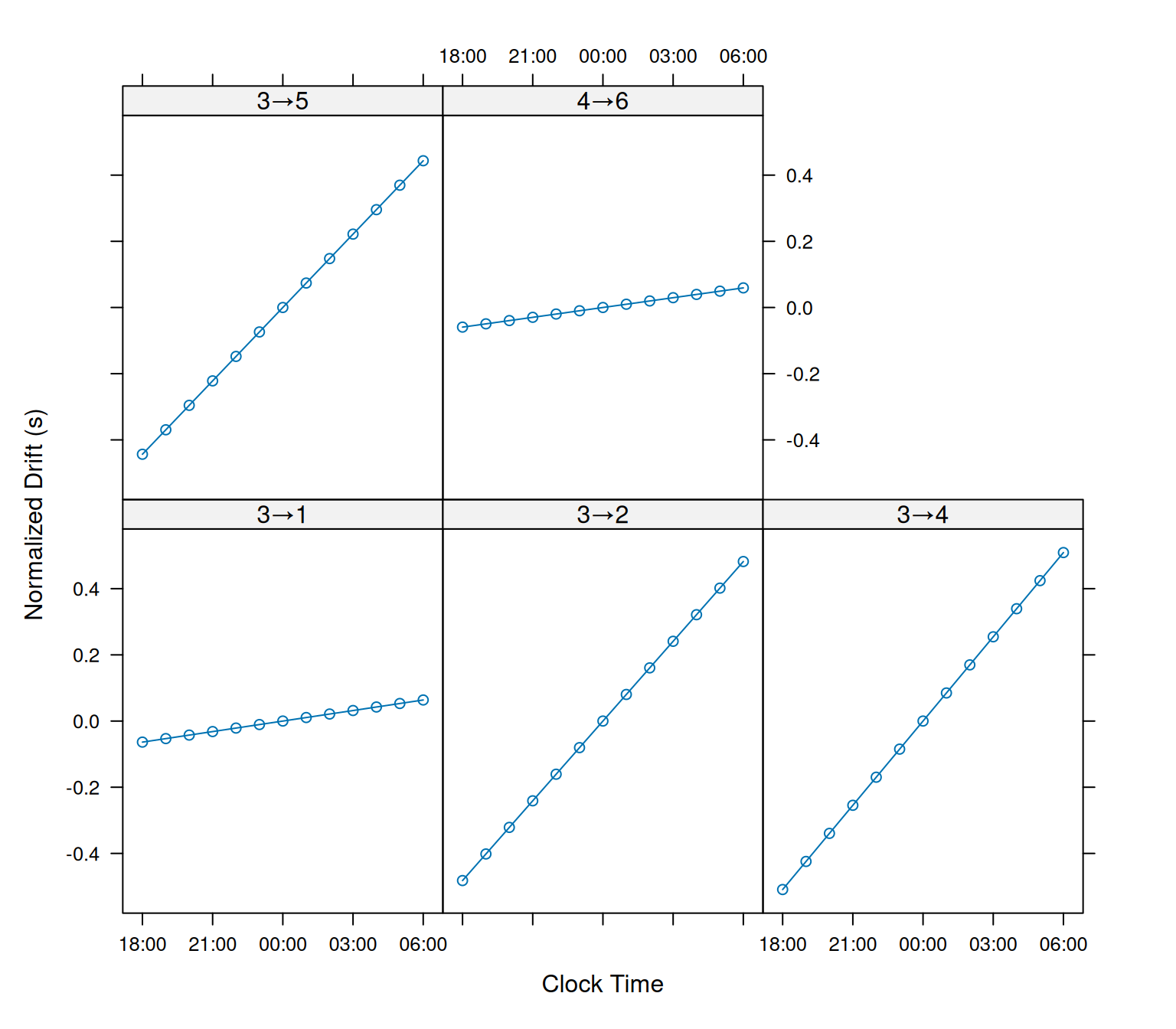
Here’s a break down of the parameters fitted by the model
- Detection sigma: The standard deviation of the detection error (for direct transmissions).
- Drift: The linear clock drift over time, seconds of additional drift per hour.
- Drift sigma: The standard deviation of the clock drift’s random walk around the linear drift line, same units as drift.
- Transmission latency: The estimated time it takes for a sync-tag to travel between a receiver pair, in seconds. This parameter captures both the distance between receivers and the speed of signal transmission.
Fitting these drift values is a messy process.
There are many parameters being estimated simultaneously by the model, so we often run into problems such as clock drift mistaken as large detection error values.
To make this easier, we opted to provide fixed values for the detection error above.
fix_sigma_det = T tells our model to treat our provided detection error parameter sigma_det = 0.01 as the truth rather than try to estimate it.
An alternative approach is to provide a fixed value for the clock drift parameter while fitting the detection error.
The key here is that its much easier to fit either of these two parameters, rather than both of them simultaneously.
Here, we’ll use the results from permute_clock_drift to guide us on setting a sensible drift error parameter
fit_drft_2 <- fit_clock_drift(
  sync_model, quiet = T,
  sigma_drift = 0.1*1e-3,# (s) Initial value for drift error (s/h)
  fix_sigma_drift = T,# Do not fit the drift error parameter
  )
print(fit_drft_2)
## --- Kaltoa receiver drift model
## Detection σ (ms) Drift (ms h⁻¹) Drift σ (ms h⁻¹)
## 3 ⟷ 1 0.0747 10.605 0.1
## 3 ⟷ 2 0.19611 80.319 0.1
## 3 ⟷ 4 0.053452 84.839 0.1
## 3 ⟷ 5 0.071724 73.898 0.1
## 4 ⟷ 6 0.81571 9.8863 0.1
## Trns. lat. (ms)
## 3 ⟷ 1 20.772
## 3 ⟷ 2 20.771
## 3 ⟷ 4 26.363
## 3 ⟷ 5 13.214
## 4 ⟷ 6 27.271
##
## Drift values
## 3 ⟷ 1 3 ⟷ 2 3 ⟷ 4 3 ⟷ 5 4 ⟷ 6
## 2021-05-08 18:00:00 0.37242 33.211 34.582 30.107 4.3173
## 2021-05-08 19:00:00 0.38305 33.291 34.667 30.181 4.3271
## 2021-05-08 20:00:00 0.39370 33.372 34.752 30.255 4.3370
## 2021-05-08 21:00:00 0.40434 33.452 34.837 30.329 4.3470
## 2021-05-08 22:00:00 0.41494 33.532 34.921 30.403 4.3569
## 2021-05-08 23:00:00 0.42554 33.613 35.006 30.477 4.3667
## 2021-05-09 00:00:00 0.43614 33.693 35.091 30.551 4.3766
## 2021-05-09 01:00:00 0.44675 33.773 35.176 30.625 4.3864
## 2021-05-09 02:00:00 0.45732 33.854 35.261 30.699 4.3962
## 2021-05-09 03:00:00 0.46795 33.934 35.346 30.773 4.4061
## 2021-05-09 04:00:00 0.47858 34.014 35.431 30.847 4.4160
## 2021-05-09 05:00:00 0.48908 34.095 35.515 30.920 4.4260
## 2021-05-09 06:00:00 0.49967 34.175 35.600 30.994 4.4359
Every telemetry array is unique, so some trial and error will have to be used to find which fitting approach works best for your dataset on hand.
Finally, lets store our fitted drift values in our KaltoaClockSync model.
# Save drift values to KaltoaClockSync model
clock_drift(sync_model) <- fit_drft_1
# Plot sync-tag diagnostics
plot(sync_model, type = 'error', layout = c(4,4))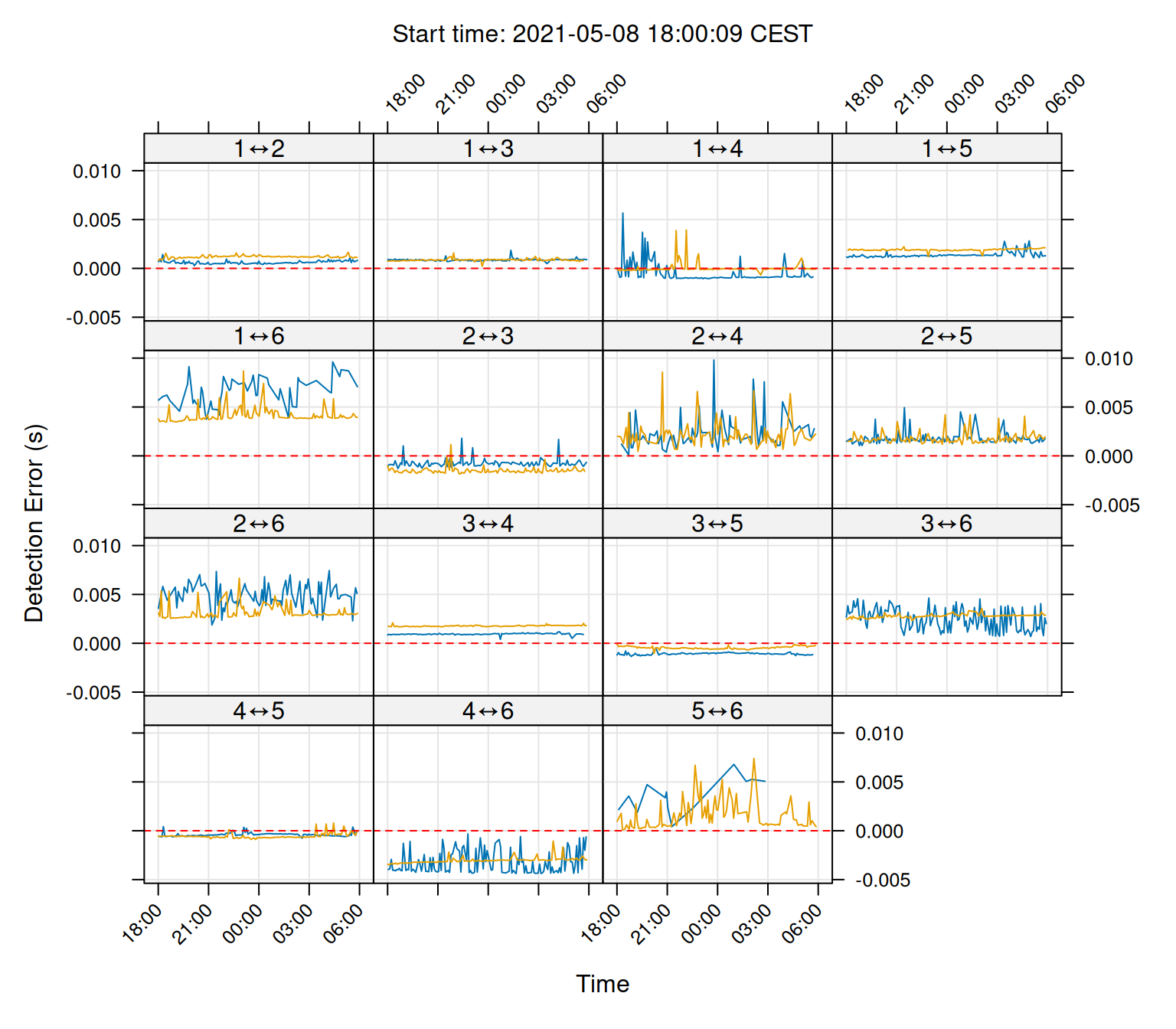
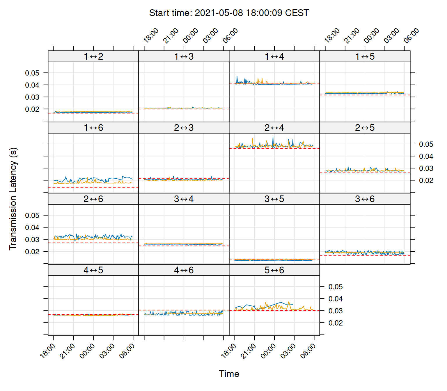
Now the sync-tag diagnostic plots show that the transmission latency is more-less constant over time. Note how some receiver pairs have a bias above or below their expected transmission latencies. These can be correct for in the next section.