1 Basic Use
paPAMv2 provides a suite of analysis options which can generally be categorized into three use cases:
- Analysis of continuous stationary sounds.
- Analysis of continuous non-stationary sounds.
- Analysis of transient sounds.
Continuous stationary sounds are those which you want to average as they don’t have well defined starting or stopping points. Generally, the processes which generate these sounds don’t substantially change over time. For example: a 10 minute long recording of an ambient soundscape, or recording of a boat engine at a fixed distance and bearing. Power spectral density, root-mean-square, and kurtosis are appropriate measurements for characterizing these types of sounds.
Continuous non-stationary sounds are continuous sounds where the sound generating process is expected to change over time. Again, these sounds don’t have clear starting or stopping points. You can think of this as a 24 hour recording of a reef where the biotic noise has unique signatures for diurnal, nocturnal, and crepuscular periods; or a recording of a moving boat which changes its loudness and timbre as its measured by a stationary vector sensor. We can use the same measurements as continuous stationary sounds here, but instead of averaging over the whole signal duration we calculate these measures in sequential time bins. The binned analysis versions of root-mean-square and kurtosis can be used here, along with a Spectrogram.
Transient sounds have a clear temporal structure. They have starting and ending points. Sounds such as shrimp snaps, fish vocalizations, or seismic survey shots are clear examples of this class. The metrics for measuring transient sounds should be robust to excess quiet periods at the start or end of the signal. Exposure, energy spectral density, and zero-to-peak are examples of transient sound measures. paPAMv2 also provides impulse kurtosis and impulse root-mean-square which are modified versions of continuous measures suitable for use in transient contexts. Finally, rise time and pulse length characterize the time-domain of transient signals.
When using paPAMv2, the available analyses are presented as check boxes on the left hand-column of the user interface. These are divided into time-domain or frequency-domain types. Broadly, frequency-domain analyses require a Fourier transformation for convert a time-series into a frequency-spectrum (changing the units of seconds into Hertz). In other words, any analysis which returns frequency information is covered by this category.
Analyses which are specifically suited for continuous or transient sounds are found under their relevant sub headers. For continuous non-stationary sounds, the binned analysis can be used. Note that these are just suggestions. No doubt users will come across sounds or use cases which don’t fit neatly into these suggested categories or use-cases.
Now that we’ve covered the types of sounds that paPAM expects, lets walk through the data processing pipeline. After raw data is collected, data processing can be broken down into four key steps as laid out below.
In the following sections, we’ll walk through how paPAMv2 is used in each of these steps.
1.1 Calibration
paPAMv2 can analyse data collected by hydrophones or vector sensors. As such, two calibration methods are provided: End-to-end and recorder and receiver sensitivity calibration. The figure below shows an overview of sensor calibration.
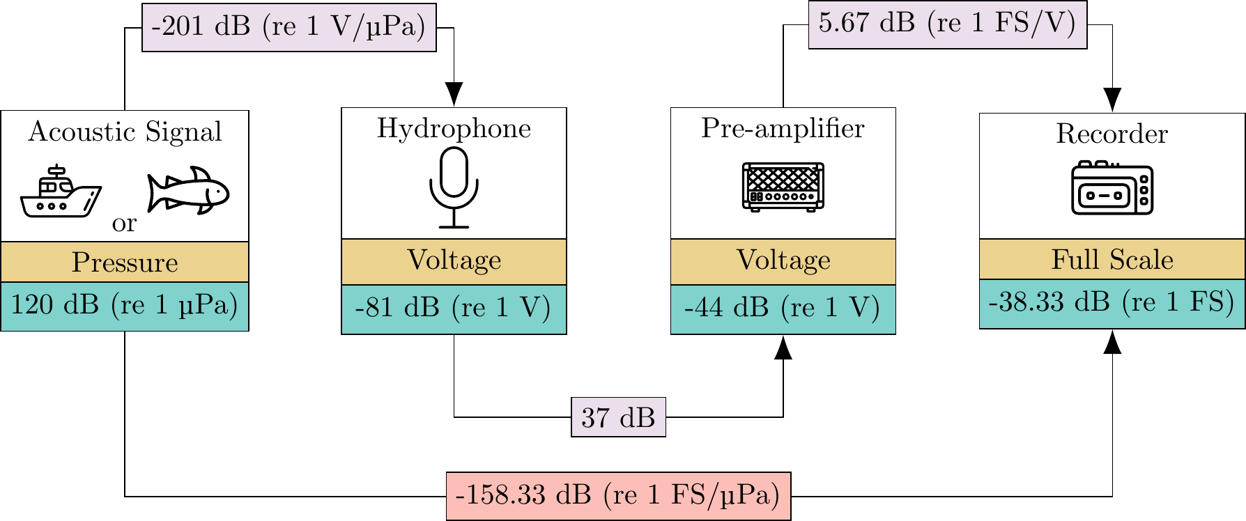
Figure 1.1: Breakdown of end-to-end sensor calibration.
The goal of calibration is to convert our digitized measurements collected by the recorder into real world units such as pressure or particle acceleration. In paPAMv2, we convert the digitized values (i.e. the raw uncalibrated data stored on your recorder) to full scale units — abbreviated by FS. Full scale units are normalized between -1 and 1, where 1 represents the loudest sound you can measure on your recorder without clipping. dBFS is a common abbreviation for dB (re FS). Hence, our end-to-end calibration units are a conversion factor between FS and real units: FS/μPa.
End-to-end calibration may be familiar to users of sountrap hydrophones; the manufacturer will simply provide a single calibration value, such as -175.2 dB (re FS/ μPa) for the soundtrap ST500. Note that soundtrap documentation provides their units in dB (re μPa/FS) while paPAMv2 expects dB (re FS/μPa); simply multiply by -1 to convert between the two decibel units.
Calibrating via recorder & receiver sensitivity is a bit more involved. For vector sensors (sensors that measure particle motion), manufacturers will make available receiver sensitivity plots which provide units such as dB (re V/μPa). These plots can be provided to paPAMv2 as an 8 column csv file: Each pair of 4 columns holds the frequency and dB for the x, y, z, and pressure channels. If your vector sensor doesn’t measure one of these channels, just leave those columns empty. Calibration units should be given in decibels with reference values set as 1 nm/s, 1 μm/s², or 1 μPa, depending if that channel is measuring velocity, acceleration, or pressure. On the user interface, a preview button is provided for the receiver sensitivity input so you can verify that your file was formatted correctly.
Next, it’s up to the user to determine the appropriate recorder gain when making measurements. Gain just refers to an amplification of the signal as it passes into your recorder. Recording devices typically have adjustable gain settings, so you’ll have to calculate a new recorder sensitivity value each time you adjust your recorder’s gain settings. Generally speaking, you should adjust your recorders gain so the loudest expected sound peak is a few dB shy of clipping. For example, -6dBFS. This will maximize the dynamic range of your recordings — i.e. give you a higher resolution measurement. However, make sure to avoid clipping at all costs. Clipped sounds (those exceeding 0dBFS) no longer hold any usable information. Setting your gain is a delicate balance between maximizing your dynamic range and minimizing the risk of clipping.
To generate a recorder sensitivity value for your chosen gain, you’ll need to playback a tone of known voltage into your recorder. The figure below provides an outline on how to do this.
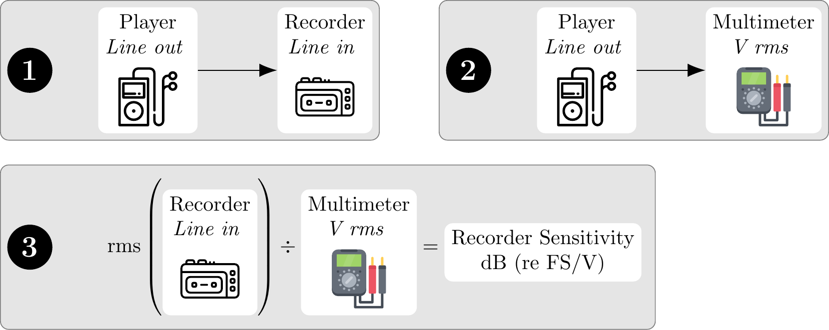
Figure 1.2: Protocol for calulating the recorder calibration constant.
- Plug a playback device into your recorder and playback a 1kHz pure tone. Record this tone.
- Next, connect the playback device to a multimeter and repeat the playback. You should set your multimeter to the appropriate root-mean-square Voltage setting. Note down the measured value.
- The recorder sensitivity is a decibel value calculated from the ratio of root-mean-square FS of the recorded tone and the root-mean-square Voltage you noted down in the previous step.
paPAMv2 provides tools to automate the creation of the calibration tone, Calibration Tools -> Calibration Tone; and calculating the recorder sensitivity value in step 3, Calibration Tools -> Recorder Sensitivity.
Some measurement systems may have an amplifier between the vector sensor and recorder. In this case, you’ll have to determine the gain of the amplifier/preamplifier and add it on to your recorder sensitivity value provided to paPAMv2.
Lastly, the recorder & receiver sensitivity calibration input was specifically designed for vector sensors which have frequency-dependent calibration data. Hydrophones, on the other hand, tend to have flat calibration curves. For recording systems which consist of a hydrophone and a recorder (with an optional preamplifier), users can calculate their own end-to-end calibration values by summing the decibel values for receiver sensitivity, amplifier gain, and recorder sensitivity. Check the earlier figure for a visual guide on how to do this correctly.
1.2 Bandpass
When analyzing bioacoustic data, we tend to only be interested in a specific frequency band. This could be the hearing range of a target species or the bandwidth of an anthropogenic sound we’re trying to characterize. Bandpass filters are used to remove sound above and below our frequency band of interest.
paPAMv2 uses Butterworth bandpass filters. Butterworth filters are great because they leave your passband (the frequency range your interested in preserving) quite flat and relatively untouched. Other bandpass filters tend to introduce ripples along your bandpass region — variable jumps in volume as you go across your bandpass frequencies. The one downside of Butterworth filters is that they don’t have particularly sharp edges. We’ll show an example of this below.
When applying a Butterworth filter, we need to set an order. For a traditional Butterworth implementation, a filter order of 1 will result in a volume drop-off of 6dB per octave as you go further outside your bandpass region. Each integer increase in order gives us an additional 6dB roll-off. We also need to note that Butterworth filters allow a little bit of dampening to seep into the edges of the passband. Selecting a higher order will minimize this effect.
Finally, bandpass filters alter the phase of your signals. For many bioacoustic applications, this is something to be avoided. The solution to filter phase offsets is quite simple… just apply a second, identical filter in the opposite direction. This will cancel out any phase offsets generated by the first filter. This is what paPAMv2 does. As a result, paPAMv2’s bandpass filters do not affect the phase information in your signal, but as the filter is applied twice, the effect of the bandpass is doubled. Thus, a bandpass filter order of 1 in paPAMv2 will result in a 12dB roll off per octave.
The figure below shows how the filter order affects the resulting bandpass in paPAMv2.
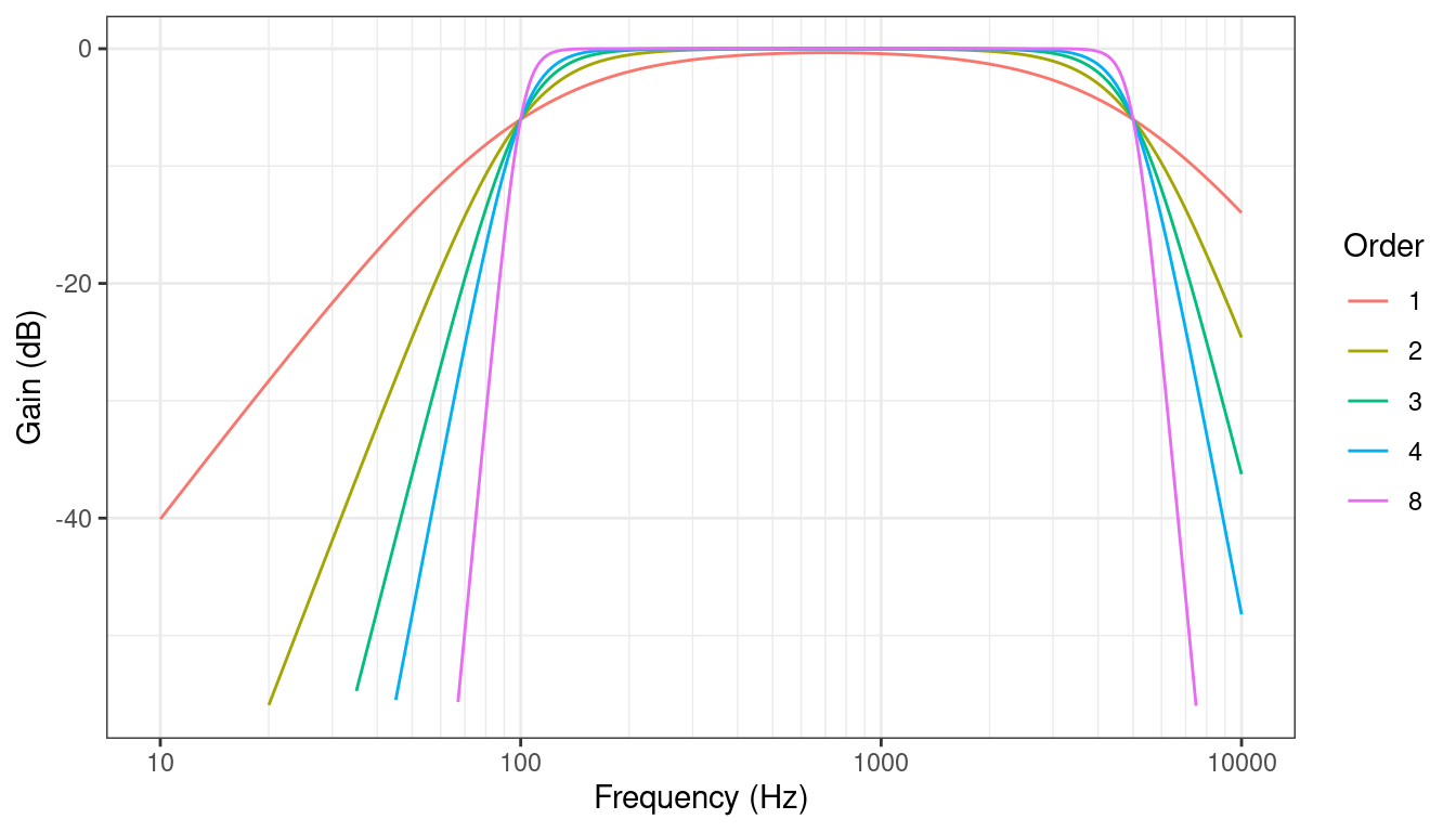
Figure 1.3: Effect of order on paPAMv2’s bandpass filter with a range of 100-5000Hz.
1.3 Analysis
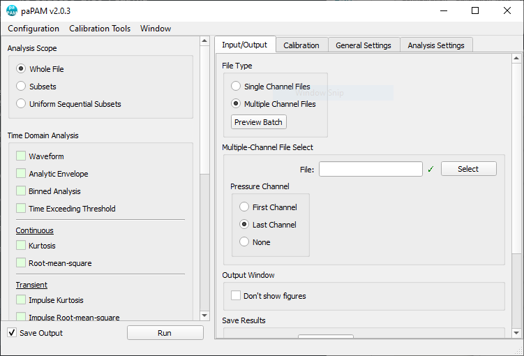
As we’ve mentioned, paPAMv2 provides all your analysis types on the left-hand column of the user interface.
Multiple options can be selected for a given run.
The remainder of the main user interface holds all the settings for the run.
To get more information on a setting, just hover your mouse over it and a tooltip should appear with a brief explanation.
If the user selects an analysis type which requires additional parameters, these options will appear in Analysis options tab.
The Run button will execute the analysis.
The analysis output is shown in the output window, in addition to being saved in an output folder.
Each analysis run also produces a log file which will be saved in the output directory.
This log file holds a copy of all the text that is produced in the output windows’s console during a run.
At the start of a run, paPAMv2 will show a call line such as papam....
This single line holds all settings used in the current run and can be copy and pasted into a terminal to replicate the analysis run.