2 Advanced Use
2.1 Directional Measures
When using a vector sensor, paPAMv2 can be used to calculate the relative bearing of sounds. These can be used for directional spectrograms, or for generating a propagation axis.
Relative bearings in paPAMv2 are given with respect to the positive direction of the x axis of the sensor. They are calculated in one of two manners:
- Particle Velocity: For a given sample with two or more measurement axes, the covariance matrix of the sample will be calculated. Singular valued decomposition will then be used to determine the bearing of the largest axis of the covariance matrix. To deal with the 180 degree ambiguity problem, the bearing pointing along the positive side of the x axis will be given.
- Sound Intensity: When a pressure channel is present, we can simply take the mean vector of sound intensity as our bearing. This does not suffer from the 180 ambiguity problem that particle velocity does. However, this method requires the pressure and particle motion channels of the vector sensor to be in phase with each other. paPAMv2 can apply phase calibrations with a receiver phase calibration file, which works analogously to the receiver magnitude calibration file.
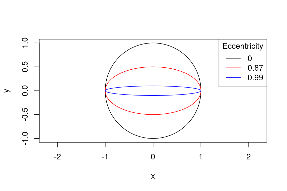
paPAMv2 also provides a measure of the quality of directionality of your signal termed eccentricity. Eccentricity is a measure of how linear or circular an ellipse is, given by
\[ e = \sqrt{1 - \frac{b}{a} },\] where \(a\) and \(b\) are the semi-major and -minor axes of the ellipse.
We provide this measure in two contexts:
Broadband eccentricity: Similar to the calculation of our particle velocity bearings, the covariance matrix of a sample is calculated. Singular valued decomposition is used to find the two largest orthogonal axes of the covariance matrix. These axes are used to calculate eccentricity. For three dimensional data sets, this is reported as free broadband eccentricity. When this calculation is applied to only data on the two axes which cover the horizontal plane, then is then referred to as horizontal broadband eccentricity.
Spectral eccentricity: For directional spectrograms, eccentricity is calculated from the Fourier transformation of the particle velocity channels. The phase and magnitude information for a given frequency across all axes are used to construct an ellipse in 3D space from which free spectral eccentricity can be calculated. Projecting this ellipse into the horizontal plane the allows for the calculation of horizontal spectral eccentricity.
Eccentricity is pretty useful when used in combination with relative bearing data. High eccentricity — close to 1 — indicates the acoustic motion of the water particles are following a very linear trajectory. When eccentricity is low, this suggests that the sound particles are moving in more circular patterns. These circular patterns can be caused by interference from other sounds or from multi-path reflections from the sound you are trying to measure. In either case, low eccentricity values suggests that the relative bearing information isn’t very reliable. When using directional spectrograms, eccentricity is always returned.
2.2 Propagation Axis
paPAMv2 allows users to create a new measurement axis on their vector sensor which points along the direction of sound propagation.
The option for this feature is found in General Settings -> Propagation Axis -> Add propagation axis.
The algorithm for this feature is as follows:
- The relative bearing of sound propagation is calculated using either sound intensity or particle velocity, specified under
General settings -> Directional Analysis. - A new axis is created in the data set, labeled
prop, which points along the relative bearing returned in step 1. - Data for this new axis is created by summing the samples from the other real axes as they are projected onto the new axis.
This is useful for getting high signal-to-noise ratio recordings of sounds which are fixed in space and able to be localized. While measurements on the pressure channel of a sensor are omni-directional, the propagation axis of the sensor will ignore sounds which are travelling orthogonal to its direction. This should result in lower ambient background noise as compared to hydrophone recordings.
2.3 Plane-wave Predicted Velocity
Under General Settings -> Soundfield Components, users can select Estimated Particle Velocity.
If a pressure channel is provided, this will use the parameters given in General Settings -> Predicted Velocity to calculate the plane-wave velocity estimation of the measured pressure values.
In other words, this provides the expected particle velocity measurement assuming an ideal far-field, deep water environment with only a single sound source.
Aside from estimating particle velocity in the absence of a vector sensor, this is also useful for checking vector sensor calibrations. In relatively far-field conditions while measuring a single source, the measured particle velocity of the vector sensor should be nearly equal to the estimated values. If the values are far off, it could be an indication that your vector sensor is not calibrated correctly.
2.4 Batch Processing
paPAMv2 supports batch processing by typing out your file names with the glob character *.
For example: C:/Users/James/Documents/Samples/trial1-*.wav.
paPAMv2 will load all files in this folder where the * character represents a string with 0 or more of any character.
This will match files like trial1-01.wav or trial1-20220101T131524.wav.
Recursive file selections are also possible.
To analyze all wav files in your Documents folder, including those in sub directories, use a double asterisk **, like C:/Users/James/Documents/**.wav.
This will match files like ~/Documents/trial_01/20220101/test_1.wav.
When batch processing on single-channel vector sensor wav files, use the preview button to make sure paPAMv2 has correctly lined up the wav files for each run.
2.5 Working with Large Files
When you only need to analyze one or a few small portions of a large file, you may select Analysis Scope -> Subsets.
A new options tab will open named Subsets where you can enter in the start and end times of each subset you want to analyze.
When doing a subset analysis, paPAMv2 will only load the portion of the file you are analyzing so it has a very small memory foot print.
In the case you want to run an analysis on a file which is too large to fit into memory, paPAMv2 provides Analysis Scope -> Uniform Sequential Subsets.
This will break your file into a series of equally sized subsets.
The user can then combine the results of the analysis afterwards.